
MRI Signal: A Complete Guide to How MRI Produces Images 2026 October
Master the MRI signal — T1, T2, proton density, pulse sequences & artifacts. 🎯 Complete guide for students, techs & registry prep.
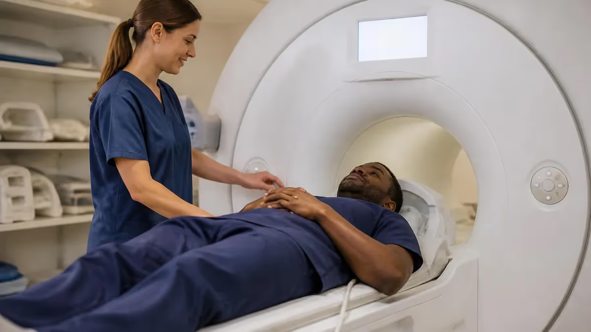
The MRI signal is the fundamental phenomenon that makes magnetic resonance imaging possible, and understanding it is essential for anyone studying radiology, preparing for the MRI registry exam, or working in a clinical imaging environment. At its core, the MRI signal arises when hydrogen protons in the body absorb radiofrequency (RF) energy and then release it as they return to equilibrium. This release of energy — carefully detected by receiver coils — encodes spatial and tissue-contrast information that computers transform into the diagnostic images clinicians rely on every day.
Hydrogen protons are ideal signal sources because they are extraordinarily abundant in the human body. Water alone accounts for roughly 60–70% of body mass, and fat tissue is nearly as proton-rich. When a patient is placed inside the bore of an MRI scanner, the powerful static magnetic field (B0) aligns these protons along the field direction, creating a net magnetization vector. Without this alignment, there would be no measurable signal to detect, because individual proton spins would cancel each other out in random orientations at room temperature.
A precisely tuned RF pulse applied at the Larmor frequency tips the net magnetization away from its equilibrium alignment. The Larmor frequency depends directly on field strength: at 1.5 Tesla it is approximately 63.87 MHz for hydrogen, and at 3 Tesla it doubles to about 127.74 MHz. When the RF pulse is turned off, protons begin to relax back toward equilibrium through two simultaneous but independent processes — longitudinal relaxation (T1) and transverse relaxation (T2) — each of which produces characteristic signal behavior that distinguishes one tissue type from another.
Manipulating these relaxation processes through the selection of pulse sequence parameters — repetition time (TR), echo time (TE), and flip angle — gives MRI technologists and radiologists an unmatched degree of tissue contrast control. A short TR combined with a short TE emphasizes T1 differences, making fat appear bright and fluid appear dark. A long TR combined with a long TE reveals T2 differences, causing fluid to appear brilliantly white while solid structures appear darker. Proton density weighting, achieved with a long TR and short TE, highlights the sheer number of protons regardless of relaxation rates.
Clinical sequences build on this foundation. Spin echo, gradient echo, inversion recovery, and echo planar imaging each exploit the signal in different ways to answer specific diagnostic questions. For example, the mri signal behavior in diffusion-weighted imaging (DWI) reflects how freely water molecules move within tissue, enabling stroke detection within minutes of symptom onset — far earlier than CT can demonstrate ischemic changes.
This guide covers every major aspect of the MRI signal: the physics of proton alignment and precession, the meaning of T1 and T2 relaxation times, how pulse sequences are designed to exploit relaxation differences, common signal artifacts and how to minimize them, and how this knowledge translates into exam success. Whether you are a student new to MRI physics or a seasoned technologist refreshing your understanding ahead of the ARRT registry, the concepts explained here will give you a solid, practical foundation for interpreting and producing high-quality MR images.
Understanding the MRI signal is not merely an academic exercise — it has direct consequences for patient safety, image quality, and diagnostic accuracy. Artifacts caused by signal misregistration, magnetic susceptibility, or motion can mimic pathology or obscure genuine disease. A technologist who grasps the underlying signal physics can proactively adjust scan parameters, select appropriate pulse sequences, and recognize artifact patterns before they degrade a study, ultimately delivering better care to patients and reducing the need for repeat examinations.
MRI Signal by the Numbers
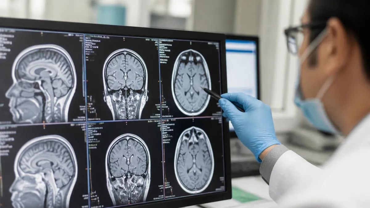
How the MRI Signal Is Created: Step by Step
Proton Alignment in B0
Precession at the Larmor Frequency
RF Excitation Pulse
Free Induction Decay (FID)
Signal Encoding (Gradients)
Image Reconstruction
T1 and T2 relaxation are the two fundamental processes that return excited protons to equilibrium after an RF pulse, and they lie at the heart of MRI contrast. T1 relaxation — also called spin-lattice or longitudinal relaxation — describes how quickly the longitudinal magnetization (Mz) recovers after being tipped away from B0.
During T1 recovery, protons transfer energy to surrounding molecules (the "lattice"). The time constant T1 is defined as the time needed for Mz to recover to approximately 63% of its equilibrium value. Fat has a short T1 (~250 ms at 1.5T) because its large, slowly tumbling molecules efficiently absorb energy from precessing protons; this makes fat appear bright on T1-weighted images.
Fluids, by contrast, have long T1 values (~2,500 ms for cerebrospinal fluid at 1.5T) because water molecules tumble very rapidly and are inefficient at absorbing proton energy. On T1-weighted images, fluid therefore appears dark. This contrast behavior is clinically invaluable: gadolinium-based contrast agents shorten T1 dramatically, causing enhancing tissue to light up brilliantly on T1-weighted post-contrast sequences. Subacute hemorrhage, which contains methemoglobin, also has a short T1 and appears bright, helping to date intracranial bleeds without contrast administration.
T2 relaxation — spin-spin or transverse relaxation — describes the dephasing of transverse magnetization (Mxy) after excitation. Individual protons within a voxel experience slightly different local magnetic fields due to interactions with neighboring protons. These minor field differences cause protons to precess at slightly different rates, gradually losing phase coherence and reducing the net transverse signal.
T2 is the time for Mxy to decay to about 37% of its initial value. Fluid has a long T2 (~200 ms) because freely tumbling water molecules do not create large local field variations; solid tissues with dense macromolecular structures, such as muscle or cortical bone, have short T2 values (~20–50 ms).
T2* (T2-star) is a related but distinct quantity that accounts for signal dephasing from both true T2 relaxation and from magnetic field inhomogeneities caused by the scanner itself or by local susceptibility differences within tissue. T2* is always shorter than T2. Gradient echo sequences are sensitive to T2* and are therefore used to detect hemosiderin deposits, calcifications, and iron — all of which shorten T2* markedly through their susceptibility effects. This makes susceptibility-weighted imaging (SWI) and T2*-weighted gradient echo sequences essential tools for detecting microbleeds and cerebral venous thrombosis.
The interplay of T1 and T2 determines the appearance of every tissue on every MRI sequence. When selecting TR and TE, the MRI technologist is essentially choosing how much T1 or T2 information to encode into image contrast. Short TR sequences allow little time for T1 recovery between pulses, so tissues with shorter T1 values (fat, subacute blood) appear relatively brighter than tissues with longer T1 values — producing T1-weighting. Long TE sequences allow more time for T2 dephasing, so tissues retaining signal longest (those with long T2, primarily fluid) appear brightest — producing T2-weighting.
Inversion recovery sequences exploit T1 differences in a powerful way by adding a 180° inversion pulse before the standard spin echo sequence. The inversion time (TI) can be chosen to null the signal from a specific tissue at the moment the 90° excitation pulse is applied. Short TI inversion recovery (STIR) suppresses fat by applying TI at the moment fat's Mz crosses the null point (~150–175 ms at 1.5T). Fluid-attenuated inversion recovery (FLAIR) nulls cerebrospinal fluid (TI ~2,000–2,200 ms at 1.5T), making periventricular lesions visible that would otherwise be obscured by the bright CSF signal.
Proton density (PD) weighting requires a long TR (allowing full T1 recovery for all tissues) and a short TE (minimizing T2 decay before signal readout). Under these conditions, signal intensity reflects primarily the local concentration of hydrogen protons rather than their relaxation properties. PD-weighted images are particularly useful in musculoskeletal MRI — for example, in evaluating meniscal tears of the knee — because they provide excellent contrast between cartilage, fluid, and fibrocartilage without the overwhelming brightness of T2-weighted fluid. Knowledge of how each weighting is achieved is a core competency tested on the ARRT MRI registry examination.
MRI Signal Weighting: T1, T2, and Proton Density Compared
T1-weighted images are produced using a short TR (300–600 ms at 1.5T) and a short TE (10–20 ms). Fat appears bright because of its short T1 relaxation time, while fluid (CSF, urine, edema) appears dark due to its long T1. Anatomy is usually well-defined, and the images have a "crisp" appearance with good soft-tissue contrast between fat-containing structures and surrounding tissues. T1-weighted sequences are the foundation for post-contrast imaging with gadolinium, where enhancing structures become hyperintense against a relatively dark background.
Clinical applications of T1 weighting include evaluation of the pituitary gland, liver lesion characterization, detection of subacute hemorrhage (methemoglobin), assessment of fatty infiltration of bone marrow, and post-contrast studies of the brain, spine, and body. Gadolinium shortens T1 dramatically in areas where the blood-brain barrier is disrupted, making T1 post-contrast the sequence of choice for detecting metastases, active demyelinating plaques, meningeal disease, and tumors throughout the body.
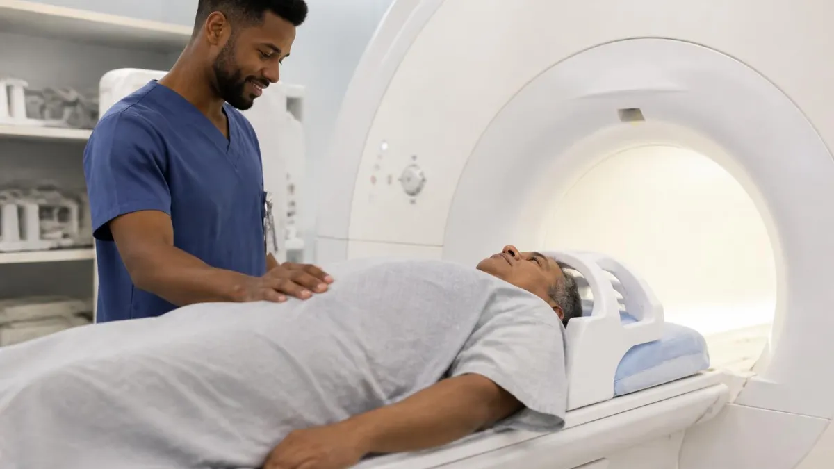
High-Field vs. Low-Field MRI Signal: Trade-Offs to Know
- +Higher field strength (3T) produces stronger net magnetization and significantly greater signal-to-noise ratio (SNR) compared to 1.5T
- +Greater SNR at 3T can be traded for finer spatial resolution, faster scan times, or both simultaneously
- +Functional MRI and spectroscopy benefit greatly from increased signal at higher field strengths
- +Higher field MRI improves detection of subtle lesions such as cortical dysplasia, small metastases, and microbleeds
- +Parallel imaging acceleration is more effective at 3T due to the inherent SNR reserve available
- +Low-field open MRI systems (0.3–0.7T) produce sufficient diagnostic signal for many routine musculoskeletal and neurological applications
- −Higher field strength increases T1 relaxation times, requiring longer TR values to achieve equivalent T1 contrast, extending scan duration
- −T2* and susceptibility artifacts are amplified at 3T, causing more pronounced distortion near air-tissue interfaces and metallic implants
- −RF energy deposition (SAR — specific absorption rate) increases with the square of field strength, imposing heating limits at 3T
- −Chemical shift artifact is doubled at 3T compared to 1.5T, requiring wider bandwidth or fat suppression on most sequences
- −Dielectric effects at 3T cause uneven B1 field distribution, producing signal intensity variations across large body parts
- −Low-field systems have lower SNR, limiting spatial resolution and making thin-slice imaging or small-structure evaluation more challenging
MRI Signal Optimization: 10-Point Technologist Checklist
- ✓Select the smallest receive coil that fully covers the region of interest to maximize SNR.
- ✓Choose TR long enough relative to tissue T1 to achieve the desired contrast weighting without excessive scan time.
- ✓Set TE short enough to capture adequate signal before T2 decay eliminates contrast in short-T2 tissues.
- ✓Apply appropriate bandwidth: narrowing bandwidth increases SNR but lengthens minimum TE and worsens chemical shift artifact.
- ✓Use fat suppression (STIR, spectral sat, or Dixon) whenever fat signal would obscure pathology or cause chemical shift artifact.
- ✓Activate parallel imaging (SENSE, GRAPPA) to reduce scan time while preserving diagnostic SNR.
- ✓Increase the number of signal averages (NSA/NEX) only when motion is not a concern, since it lengthens scan time proportionally.
- ✓Maximize field of view only as large as necessary — smaller FOV with the same matrix size reduces voxel dimensions and improves resolution.
- ✓Position the patient at isocenter of the magnet to ensure the most homogeneous B0 field and best shimming performance.
- ✓Review the shimming report and run additional localized shim procedures for challenging regions such as the posterior fossa or pelvis.
The SNR Equation Every MRI Tech Should Know
Signal-to-noise ratio (SNR) is proportional to voxel volume × √(number of averages) × √(scan time). Doubling the number of signal averages increases SNR by only ~41% while doubling scan time — making coil selection, field strength, and voxel size far more efficient levers for improving image quality than simply averaging more acquisitions.
MRI signal artifacts arise when the raw data in k-space does not accurately represent the true spatial distribution of protons in the patient's body. Understanding these artifacts is critically important for both producing diagnostic-quality images and avoiding misdiagnosis. Some artifacts mimic pathology; others merely degrade image quality. The most commonly encountered artifacts on the ARRT MRI registry exam include motion artifact, aliasing (wrap-around), chemical shift, magnetic susceptibility, Gibbs ringing, and magic angle effects.
Motion artifact is perhaps the most clinically significant because it is ubiquitous and can render images non-diagnostic. It appears as ghosting — repeated copies of moving structures smeared across the image in the phase-encoding direction. Respiratory motion, cardiac pulsation, vascular pulsatility, peristalsis, and voluntary patient movement all contribute.
Mitigation strategies include breath-hold imaging, respiratory triggering or gating, cardiac gating, saturation bands to suppress signal from moving structures outside the region of interest, and navigator echo techniques that continuously track diaphragm position. For uncooperative patients, very fast sequences such as single-shot echo planar imaging (EPI) or HASTE can essentially freeze motion entirely.
Aliasing (wrap or fold-over artifact) occurs when anatomy outside the prescribed field of view is assigned incorrect spatial positions and folds onto the image. This happens because the Fourier transform treats signal periodically — anatomy beyond the FOV edge is misregistered to the opposite side. Corrections include increasing the FOV (at the cost of reduced resolution if the matrix is not also increased), applying saturation bands over the aliased tissue, enabling oversampling in the phase direction, or swapping phase and frequency directions so that the aliasing occurs across a dimension that does not obscure the anatomy of interest.
Chemical shift artifact occurs at fat-water interfaces because fat protons resonate at a slightly lower frequency than water protons — approximately 3.5 parts per million (ppm) lower, which corresponds to 220 Hz at 1.5T and 440 Hz at 3T. The frequency-encoding gradient assigns spatial positions based on resonance frequency, so fat is misregistered relative to water by a number of pixels proportional to the chemical shift divided by the receiver bandwidth per pixel.
At narrow bandwidths, the misregistration can be several pixels wide, creating a dark band on one side of fat-containing structures and a bright band on the other. Using wider bandwidth, fat suppression, or a water-only sequence (Dixon method) eliminates this artifact.
Magnetic susceptibility artifact arises from local distortions of the B0 field caused by differences in magnetic susceptibility between adjacent materials. Air-tissue interfaces (sinuses, lung-liver border), calcifications, hemorrhagic products containing hemosiderin or deoxyhemoglobin, and metallic implants all create susceptibility effects. The severity is much greater on gradient echo sequences (which are T2*-sensitive) than on spin echo sequences (where the 180° refocusing pulse partially corrects susceptibility dephasing). Reducing TE, increasing receiver bandwidth, and switching from GRE to SE or FSE can all reduce susceptibility artifact, though some susceptibility sensitivity is actually desirable for detecting microbleeds or iron deposition.
Gibbs ringing (also called truncation artifact or ringing artifact) appears as alternating bright and dark bands near sharp signal boundaries — most commonly at the edge of the brain near the skull, or at the spinal cord-CSF interface. It results from the finite number of phase-encoding steps used to sample k-space; sharp boundaries contain high spatial frequency information that is truncated when not enough k-space lines are acquired. Increasing the number of phase-encoding steps (larger matrix) reduces Gibbs ringing, as does applying a low-pass filter during reconstruction, although filtering slightly reduces sharpness.
The magic angle effect is a tissue-specific artifact rather than an imaging artifact per se. In fibrous tissues such as tendons, ligaments, and menisci, T2 relaxation time is anisotropic — it depends on the orientation of the collagen fibers relative to B0.
When a tendon is oriented at approximately 55° to B0 (the "magic angle"), dipole-dipole interactions between water protons bound to collagen are minimized, artificially prolonging T2 and causing the tendon to appear abnormally bright on T1 and PD sequences with short TE. Radiologists and technologists must recognize that this brightening does not represent true tendinopathy; changing patient positioning or using sequences with longer TE eliminates the effect.
You can continue preparing with the open mri locations near me, which includes answer explanations for every question.
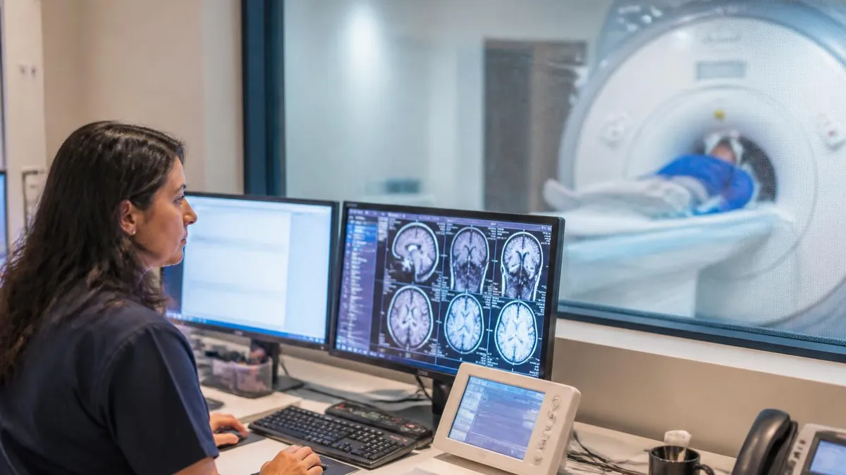
Specific Absorption Rate (SAR) — the rate at which RF energy is deposited in tissue — increases with the square of B0 field strength and directly with flip angle. At 3T, SAR limits are reached much more quickly than at 1.5T, especially during fast spin echo sequences with many 180° refocusing pulses. Always monitor SAR levels displayed by the scanner and reduce flip angles, increase TR, or reduce the number of slices per TR if SAR limits are exceeded to prevent patient tissue heating.
Preparing for the ARRT MRI registry examination requires a thorough understanding of MRI signal physics, and the topics covered in this guide represent some of the highest-yield content on the exam. The registry tests not just factual recall but the ability to apply signal principles to clinical scenarios — for example, recognizing which pulse sequence parameter to change when an image shows chemical shift artifact, or identifying why a lesion is bright on both T1 and T2 sequences. Building this applied understanding is the key difference between candidates who pass on the first attempt and those who struggle.
The registry examination blueprint divides content into several major domains, with MRI physics and instrumentation typically accounting for a significant portion of the total questions. Within the physics domain, you should be confident explaining the Larmor equation and its clinical implications, describing longitudinal and transverse relaxation and how each is measured, comparing spin echo and gradient echo pulse sequences, explaining the purpose of each gradient axis, and defining k-space and how different regions contribute to image contrast versus resolution. These are not obscure topics — they appear on virtually every registry preparation question set.
When studying relaxation times, use tissue-specific anchor values to build your mental model. At 1.5T: fat T1 ≈ 250 ms, muscle T1 ≈ 870 ms, white matter T1 ≈ 780 ms, gray matter T1 ≈ 920 ms, CSF T1 ≈ 2,500 ms. For T2: muscle ≈ 50 ms, white matter ≈ 90 ms, gray matter ≈ 100 ms, CSF ≈ 200 ms.
Knowing these values allows you to predict image contrast for any combination of TR and TE and to explain why tissues appear bright or dark on a given sequence — a question type that appears frequently on the registry.
Pulse sequence recognition is another high-yield registry skill. Given an image description or set of scan parameters, you should be able to identify whether the sequence is T1-weighted spin echo, T2-weighted fast spin echo, STIR, FLAIR, gradient echo, or echo planar imaging. Key distinguishing features include the shape of the signal readout (single echo vs. echo train vs. gradient reversal), the presence or absence of 180° refocusing pulses, the TR and TE ranges, and the specific tissue contrasts produced. Practice reading parameter tables and associating them with sequence types and clinical applications.
K-space understanding is frequently tested in ways that trip up unprepared candidates. The center of k-space stores low spatial frequency data and determines overall image contrast and signal intensity. The periphery of k-space stores high spatial frequency data and determines edge detail and spatial resolution.
Partial Fourier imaging (acquiring only a portion of k-space and mathematically estimating the rest) reduces scan time but degrades SNR and resolution if too much data is omitted. Keyhole imaging and PROPELLER (periodically rotated overlapping parallel lines with enhanced reconstruction) are advanced k-space strategies that reduce motion sensitivity — topics increasingly appearing on modern registry exams.
Safety topics related to MRI signal generation are also testable. The three major MRI safety concerns are static magnetic field effects (projectile hazard, magnetic torque on implants), time-varying gradient fields (peripheral nerve stimulation, loud acoustic noise), and RF energy deposition (heating, SAR limits). Technologists must screen patients for implanted devices, understand conditional versus non-conditional implant labeling, and know how to modify scan parameters to stay within safe SAR thresholds. The intersection of signal physics and patient safety — for example, understanding why shorter TE reduces SAR in some sequences — is a sophisticated topic that distinguishes high-scoring candidates.
Finally, remember that the registry rewards depth of conceptual understanding over breadth of memorized facts. When you encounter a challenging question about an unfamiliar artifact or sequence variant, apply first principles: where is the signal coming from, how is it being manipulated by TR and TE, and what happens to proton dephasing and rephasing under these conditions?
Candidates who internalize this framework can reason through unfamiliar scenarios rather than relying solely on memorized associations, giving them a significant advantage on exam day. Use the practice quizzes and study resources on PracticeTestGeeks.com consistently in the weeks leading up to your exam to reinforce both recall and reasoning.
Practical mastery of MRI signal concepts begins with connecting abstract physics to everyday scanner operation. Every time you set up a scan, challenge yourself to predict how the chosen TR and TE will affect tissue contrast before acquiring the first image. Ask: will fluid be bright or dark? Will fat need to be suppressed? Is the TE short enough to capture adequate signal from short-T2 structures like fibrocartilage or cortical bone? This habit of prediction-and-verification rapidly builds the intuition that separates proficient technologists from truly expert ones.
When troubleshooting image quality problems, always start with SNR. Low SNR manifests as a grainy, noisy appearance and can result from a coil too distant from the anatomy, a voxel size too small for the available signal, too few signal averages, or a TR so short that longitudinal magnetization never fully recovers. Systematically work through each variable: coil selection and positioning first (highest impact, no time cost), then voxel size, then averages, then TR adjustment. Document your solutions — over time, you will build a personal reference library of optimizations for common problem scenarios in your practice setting.
For those preparing for the ARRT registry, a structured study schedule significantly improves outcomes. Spend the first two weeks reviewing fundamental physics: proton behavior, relaxation, and the Larmor equation. Weeks three and four should cover pulse sequences in detail — spin echo, inversion recovery, gradient echo, and EPI.
Devote week five to artifacts: learn to identify each artifact type from its appearance and understand the corrective parameter change. Week six should focus on safety (SAR, gradient limits, implant screening) and any remaining weak areas identified by practice testing. Reserve the final week exclusively for timed practice examinations to build test-taking stamina and time management skills.
Active retrieval practice — answering questions without looking at notes — is far more effective for long-term retention than passive re-reading. After studying each topic section, close your notes and write down everything you remember. Then check what you missed and pay special attention to those gaps in your next review session. Spaced repetition (reviewing material at increasing intervals as it becomes more familiar) compounds this benefit by ensuring that well-learned material takes less study time, freeing capacity for areas that need more attention.
Clinical shadowing or observation hours in an MRI department provide irreplaceable context for exam preparation. Watching an experienced technologist explain why they chose STIR over spectral fat saturation for a patient with dental hardware, or how they adjusted gradient parameters to reduce peripheral nerve stimulation in an obese patient, connects textbook physics to real decision-making in ways that no study guide can fully replicate. If your program includes clinical rotations, treat each observation opportunity as a physics seminar with real-time feedback.
Group study can be remarkably effective for mastering MRI signal concepts because explaining a concept to someone else forces you to identify and fill gaps in your own understanding. Organize study groups of three to five peers, assign each member a topic to teach in a short presentation, and critique each other's explanations for accuracy and completeness. Topics particularly well-suited to this approach include the mechanism of fat suppression techniques, the distinction between T2 and T2* relaxation, the relationship between k-space sampling and image properties, and the principles of parallel imaging.
Finally, maintain perspective on the purpose of this knowledge. Understanding the MRI signal is not just about passing an examination — it directly affects patient care. A technologist who recognizes that a subtle bright T1 signal in the posterior fossa represents methemoglobin rather than a technical artifact helps clinicians detect subacute hemorrhage.
One who immediately identifies chemical shift artifact at the renal hilum prevents a pseudolesion from being mistaken for an adrenal mass. This clinical relevance makes MRI physics one of the most rewarding subjects in the entire radiology curriculum — it is knowledge that translates directly into diagnostic value every single day of a technologist's career.
MRI Questions and Answers
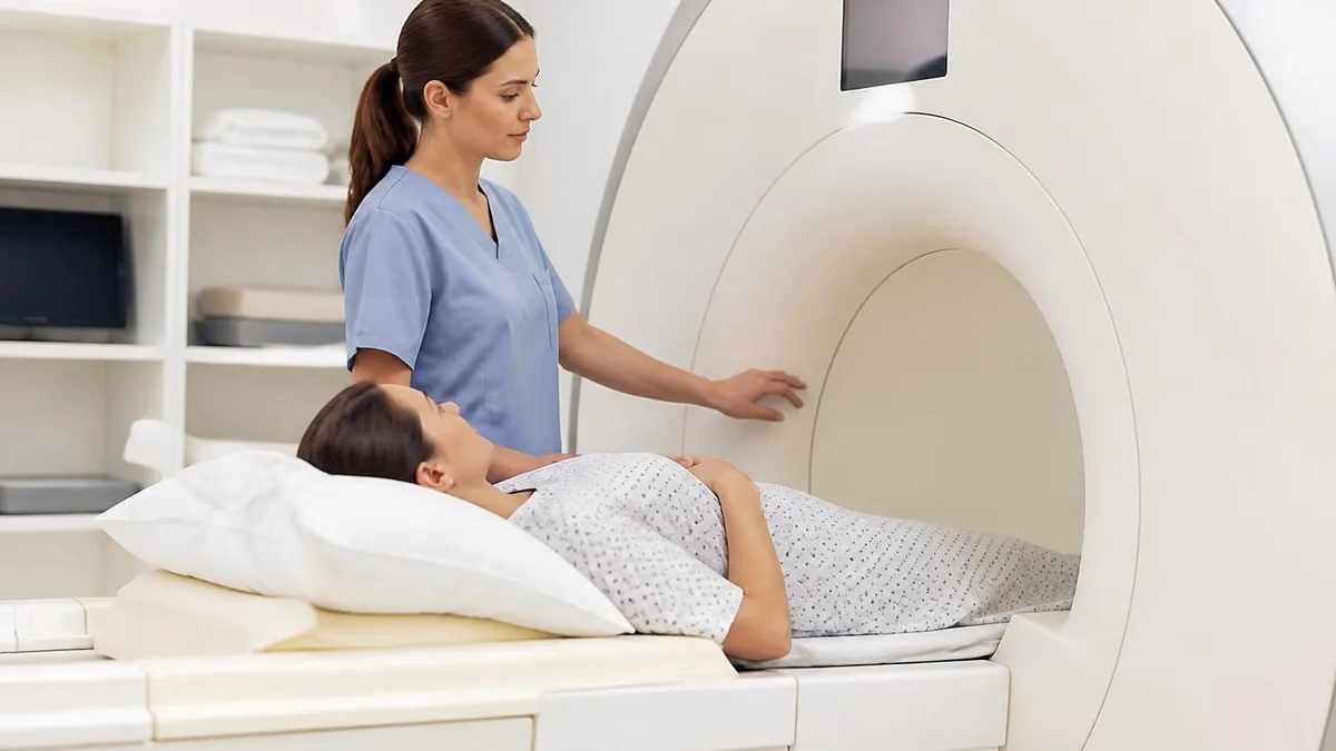
DWI MRI: Diffusion-Weighted Imaging Explained (2026 Guide)
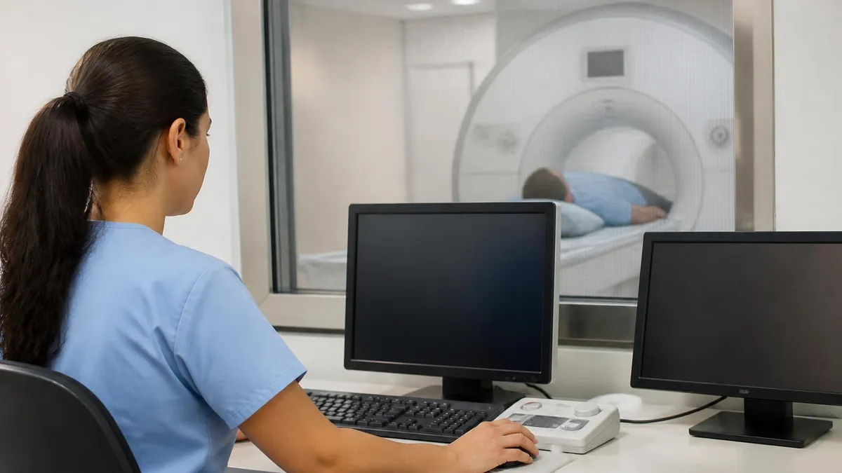
Side Effects of Brain MRI: Understanding Risks, Safety, and What Every Patient Should Know
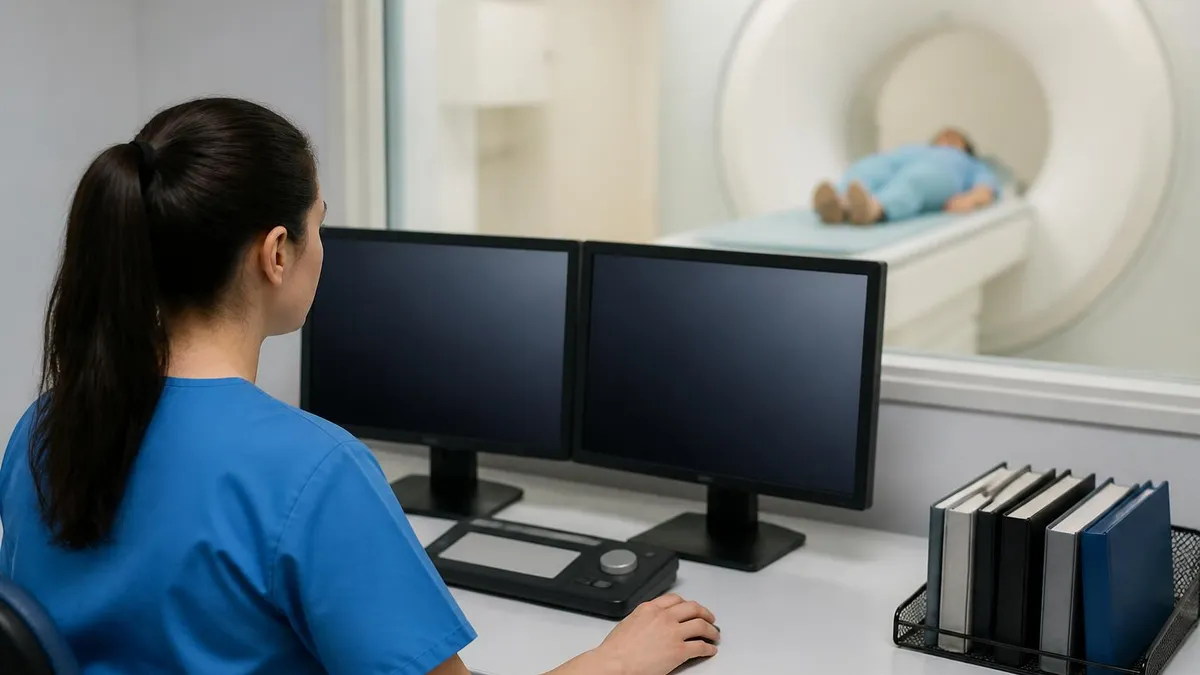
MRI Lumbar Spine Without Contrast: Complete Guide to the Scan, What It Shows, and How to Prepare
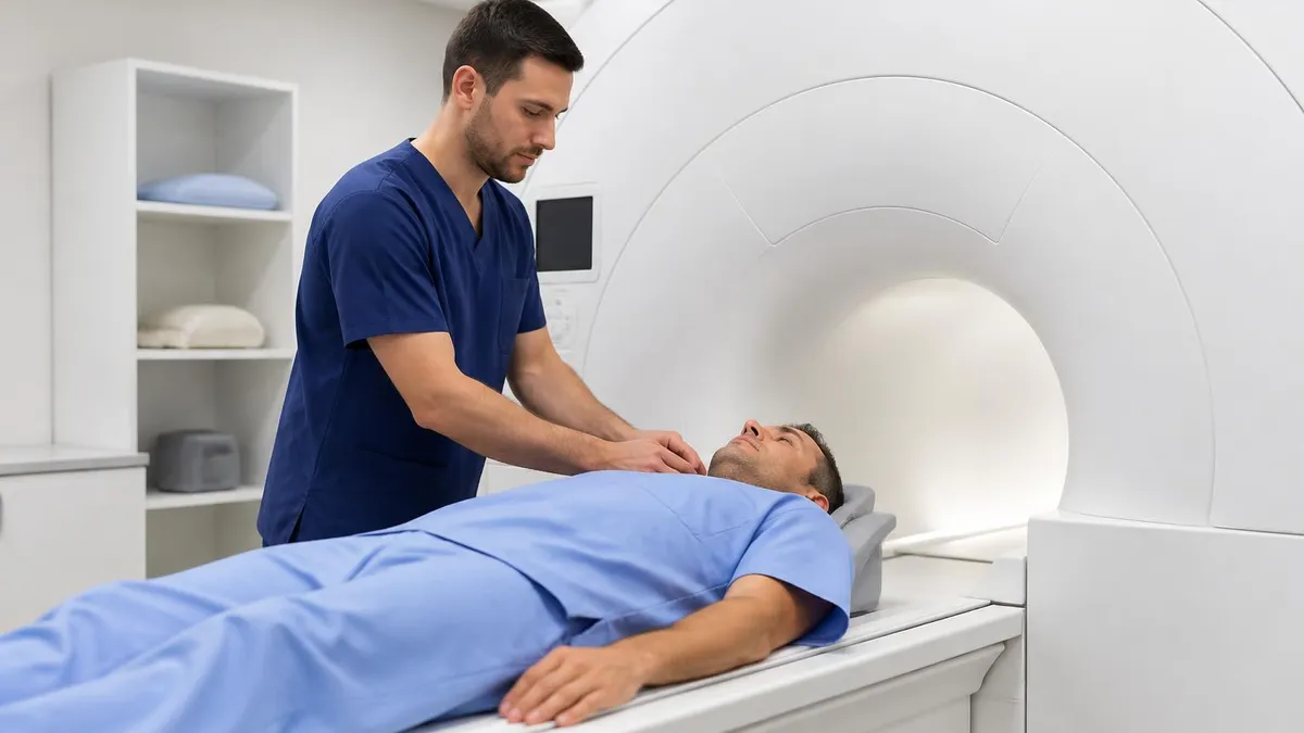
MRI History: From Nuclear Resonance to Modern Scanners
MRI of Cervical Spine: Complete Guide to Imaging, Anatomy, Pathology, and Patient Preparation
About the Author

Medical Laboratory Scientist & Clinical Certification Expert
Johns Hopkins UniversityDr. Sandra Kim holds a PhD in Clinical Laboratory Science from Johns Hopkins University and is certified as a Medical Technologist (MT) and Medical Laboratory Scientist (MLS) through ASCP. With 16 years of clinical laboratory experience spanning hematology, microbiology, and molecular diagnostics, she prepares candidates for ASCP board exams, MLT, MLS, and specialist certification tests.
Join the Discussion
Connect with other students preparing for this exam. Share tips, ask questions, and get advice from people who have been there.
View discussion (8 replies)