How to Use Excel: Formulas, Functions & Tips

You've opened a blank spreadsheet and you're staring at a grid of empty cells. Don't worry—Microsoft Excel looks intimidating at first, but once you get the basics down, it becomes one of the most powerful tools you'll ever use. Whether you're tracking expenses, analyzing sales data, or building a project timeline, Excel handles it all.

This guide walks you through everything from entering your first number to writing formulas that do the heavy lifting for you. We'll cover the interface, core functions, formatting tricks, and some genuinely time-saving shortcuts. By the end, you won't just know how to use Excel—you'll know how to use it well.

Understanding the Excel Interface

When you open Excel, you see a workbook made up of worksheets—those tabs at the bottom. Each worksheet is a grid of rows (numbered 1, 2, 3…) and columns (labeled A, B, C…). The intersection of a row and column is a cell, identified by its column letter and row number, like A1 or D7.

At the top, the Ribbon groups commands into tabs: Home, Insert, Page Layout, Formulas, Data, Review, and View. You'll live in the Home and Formulas tabs most of the time. The formula bar runs just above the grid—it shows you exactly what's in the selected cell, including any formula.

One thing beginners often miss: clicking a cell and seeing a value doesn't mean it's a raw number. It might be a formula that calculates to that value. Always check the formula bar if something looks off.

Entering and Formatting Data

Click any cell and start typing. Press Enter to move down, Tab to move right. To edit a cell you've already filled, press F2—much faster than double-clicking.

Excel auto-detects data types. Type a number and it right-aligns; type text and it left-aligns. Dates get their own treatment—Excel stores them as serial numbers internally, which is why date math (like calculating days between two dates) works so cleanly.

To format cells, select them and use the Home tab. You can apply currency, percentage, or date formats with one click. For more control, hit Ctrl+1 to open the Format Cells dialog. Here you can set decimal places, choose a date format, add a custom number mask—almost anything.

A few formatting habits that'll save you later: keep headers in row 1, use a consistent date format throughout, and avoid merged cells if you plan to sort or filter data (merged cells break both features).

Writing Your First Formulas

Every formula in Excel starts with an equals sign (=). Type =2+2 and press Enter—you get 4. Type =A1+B1 and you get the sum of whatever's in those two cells. That's the core idea: formulas reference cells, and when those cells change, the formula updates automatically.

The most-used functions are SUM, AVERAGE, COUNT, MAX, and MIN. They work like this:

• =SUM(A1:A10) — adds everything from A1 to A10
• =AVERAGE(B2:B20) — gives you the mean
• =COUNT(C1:C50) — counts cells that contain numbers
• =MAX(D1:D100) and =MIN(D1:D100) — highest and lowest values

The colon notation (A1:A10) means a range—all cells from A1 through A10. You can also select multiple non-adjacent cells with a comma: =SUM(A1,C1,E1).

When you copy a formula to another cell, Excel adjusts the references automatically. This is called relative referencing. If you want a reference to stay fixed—say, always pointing to a tax rate in cell B1—add dollar signs: =$B$1. That's an absolute reference, and it won't shift when copied.

VLOOKUP and XLOOKUP

Once you've got formulas down, vlookup excel and its successor XLOOKUP open up a whole new level of data work. VLOOKUP searches a column for a value and returns something from the same row. The syntax is:

=VLOOKUP(lookup_value, table_array, col_index_num, [range_lookup])

Say you have a product list in columns A–C (ID, Name, Price). To find the price of product ID 1042, you'd write:

=VLOOKUP(1042, A:C, 3, FALSE)

The FALSE at the end means exact match—you almost always want this. Leave it out or use TRUE and you'll get approximate matches, which is only useful for sorted numeric ranges like tax brackets.

VLOOKUP has a known limitation: it only looks to the right. If your lookup column isn't the leftmost column in your range, it won't work. That's where XLOOKUP comes in—it's Excel's newer, more flexible replacement:

=XLOOKUP(lookup_value, lookup_array, return_array)

XLOOKUP can look left, return multiple columns at once, and handles errors more gracefully. If you're on Microsoft 365 or Excel 2019+, use XLOOKUP. For compatibility with older files, stick with VLOOKUP.

IF Statements and Logical Functions

The IF function lets Excel make decisions. The structure is simple:

=IF(condition, value_if_true, value_if_false)

Example: =IF(C2>=60, "Pass", "Fail") returns "Pass" if C2 is 60 or above, "Fail" otherwise. You can nest IFs for multiple conditions, but nested IFs get messy fast. For cleaner multi-condition logic, use IFS:

=IFS(C2>=90,"A", C2>=80,"B", C2>=70,"C", C2>=60,"D", TRUE,"F")

Pair IF with AND or OR to check multiple conditions at once. =IF(AND(B2>100, C2="Active"), "Bonus", "No Bonus") only returns "Bonus" when both conditions are true.

Sorting, Filtering, and Tables

Raw data becomes useful when you can slice it. Sorting is as simple as clicking a column header and hitting the Sort A→Z or Z→A button in the Data tab. For multi-level sorts (sort by department, then by name within each department), use Data → Sort → Add Level.

Filtering lets you show only rows that meet certain criteria. Select your data and press Ctrl+Shift+L to add filter dropdowns to your headers. Click a dropdown and you can filter by value, date range, number range, or custom text criteria.

For anything more than a one-off sort or filter, convert your data to a Table. Click anywhere in your data and press Ctrl+T. Tables automatically expand when you add rows, apply consistent formatting, and make formulas cleaner (you reference column names like [Price] instead of column letters). They're one of Excel's most underused features.

Pivot Tables: The Real Power Move

If you work with large datasets, pivot tables will change how you think about data analysis. A pivot table summarizes thousands of rows into a compact, interactive summary—by category, date, region, or any other field you choose.

To create one: click anywhere in your data, go to Insert → PivotTable, and click OK. A new sheet opens with a field list on the right. Drag fields to the Rows, Columns, Values, and Filters areas. Want total sales by month? Drag "Month" to Rows and "Sales" to Values. Done. Want to break that down by product? Drag "Product" to Columns.

Pivot tables don't change your source data—they just give you a different view of it. Refresh the pivot (right-click → Refresh) whenever the source data changes. For quick charts from a pivot, use Insert → PivotChart—you get a chart that updates when the pivot updates.

Essential Keyboard Shortcuts

Speed matters. These shortcuts will cut your Excel time significantly:

• Ctrl+C / Ctrl+V — copy/paste (everyone knows this one)
• Ctrl+Z / Ctrl+Y — undo/redo
• Ctrl+Home / Ctrl+End — jump to beginning or last used cell
• Ctrl+Arrow keys — jump to the edge of a data range
• Ctrl+Shift+Arrow — select to the edge of a range
• Ctrl+D — fill down (copy the cell above into selected cells)
• Alt+Enter — line break inside a cell
• F4 — repeat last action, or toggle absolute/relative reference in a formula
• Ctrl+; — insert today's date
• Alt+= — auto-sum selected range

Learn these gradually—pick two or three each week. Within a month, your hands will reach for them automatically.

Conditional Formatting

Conditional formatting applies visual formatting—colors, icons, data bars—based on cell values. It's a quick way to spot outliers, trends, and problem areas without reading every number.

Select your data, go to Home → Conditional Formatting. You can highlight cells above/below a value, apply a color scale (green-yellow-red gradient), add data bars inside cells, or use icon sets (arrows, traffic lights). For custom rules—like highlighting rows where a project is overdue—use "New Rule" and write your own formula.

One practical use: apply a color scale to a column of scores. The top scores go green, the bottom go red, and everything in between gets shades of yellow. At a glance, you see the distribution without any analysis.

Working with Multiple Sheets

Workbooks can hold dozens of sheets. Right-click any sheet tab to insert, delete, rename, move, or copy it. You can reference cells from other sheets in formulas: =Sheet2!B3 pulls the value from B3 on Sheet2.

For a formula that spans sheets—say, summing January through December sheets—use a 3D reference: =SUM(January:December!B5) adds cell B5 from every sheet between January and December tabs. Make sure the tabs are in order and the cell location is the same on each sheet.

Keep sheets organized: use clear names, group related data on one sheet, and use a summary sheet that pulls key numbers from the others. This structure makes workbooks much easier to maintain as they grow.

Common Mistakes to Avoid

A few errors trip up almost everyone starting out:

Hard-coding values in formulas. If your formula is =A1*0.08 for a tax rate, put that 0.08 in a cell (say, B1) and reference it: =A1*B1. When the tax rate changes, you update one cell instead of hunting through every formula.

Using VLOOKUP when the lookup column isn't leftmost. This forces you to restructure your data. Use INDEX/MATCH or XLOOKUP instead—both work regardless of column order.

Mixing data types in a column. A mix of text and numbers in the same column breaks sorting, filtering, and aggregation functions. Keep columns clean: numbers in number columns, text in text columns.

Not saving backups. Excel's autosave (in Microsoft 365) helps, but enable it explicitly and periodically save a versioned copy for anything important. Nothing's worse than losing an afternoon's work to a crash.

Data Validation and Drop-Down Lists

If you're building a spreadsheet others will use, data validation prevents bad input. You can restrict a cell to accept only numbers in a certain range, dates within a window, or text from a predefined list.

To add a drop-down list: select the cell(s), go to Data → Data Validation, set Allow to "List", and type your options separated by commas (or reference a range). Now users click an arrow to choose from your list instead of typing freeform—no more typos, no more inconsistent entries.

For numeric validation: set Allow to "Whole number" or "Decimal", then set a minimum and maximum. Add an error message in the "Error Alert" tab so users know what went wrong if they enter something invalid.

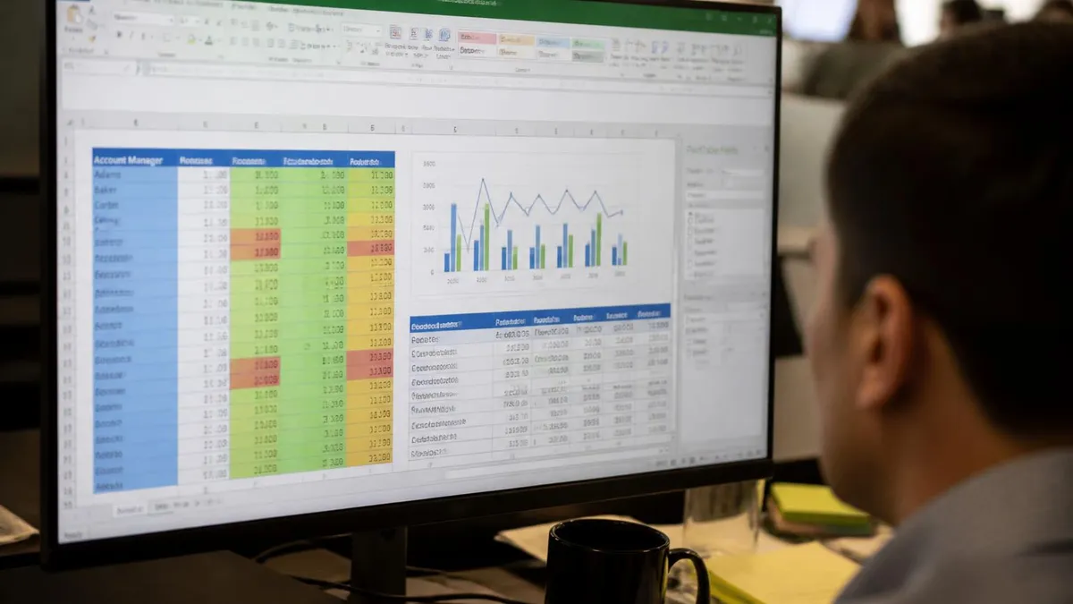
Charts and Data Visualization

Excel's charting tools turn numbers into visuals that tell a story. Select your data (including headers), go to Insert → Recommended Charts, and Excel suggests chart types based on your data structure. Take its suggestions or browse the full chart library.

A few chart-type guidelines: use line charts for trends over time, bar/column charts for comparing categories, pie charts for parts of a whole (but only when you have fewer than 6 slices—anything more gets unreadable), and scatter plots for relationships between two variables.

After inserting a chart, click it and use the Chart Design and Format tabs to adjust colors, labels, titles, and axis ranges. Right-click any element for more options. One useful trick: click a chart and press F11 to immediately move it to a dedicated chart sheet at full size—great for presentations.

Protecting Your Work

When sharing workbooks, you often want to prevent accidental edits to formulas or key cells. Excel lets you lock specific cells and then protect the sheet.

By default, all cells are marked as "Locked," but locking only takes effect when sheet protection is on. The workflow: first unlock the cells users should be able to edit (select them, press Ctrl+1, go to Protection tab, uncheck Locked). Then go to Review → Protect Sheet and set a password. Now only the unlocked cells are editable—everything else is read-only.

To protect the entire workbook structure (so users can't add, delete, or rename sheets), use Review → Protect Workbook. You can combine both protections for a fully locked-down file.

Using Excel for Real Projects

The gap between knowing Excel features and using Excel effectively is practice on real problems. Here are some starter projects that teach multiple skills at once:

Personal budget tracker: Columns for date, category, description, and amount. A summary section using SUMIF to total by category. Conditional formatting to flag large expenses. This teaches ranges, SUMIF, and formatting in one shot.

Grade calculator: Student names in column A, assignment scores across columns B–F, weighted average in column G using a formula like =SUMPRODUCT(B2:F2, $B$1:$F$1)/SUM($B$1:$F$1) where row 1 holds the weights. Letter grades in column H using IFS. This teaches absolute references, SUMPRODUCT, and nested logic.

Sales dashboard: Raw transaction data on one sheet. A pivot table on another sheet summarizing by product and month. A chart tied to the pivot. Slicers for filtering. This is a full mini-project covering tables, pivots, charts, and interactivity.

Each project will surface questions you didn't know you had—and answering those questions is how you actually learn Excel rather than just reading about it.

Putting It All Together

Learning how to use Microsoft Excel isn't about memorizing every function—it's about building a mental model of how the pieces fit. Cells hold data or formulas. Formulas reference cells. Functions are pre-built formulas for common calculations. Tables organize data and make formulas safer. Pivot tables summarize data without changing it. Charts visualize it.

Start with whatever task is in front of you. Entering a budget? Learn SUM and basic formatting. Analyzing sales data? Tackle pivot tables. Building a tool for your team? Explore data validation, protection, and drop-down lists. Real problems are the fastest teacher.

If you want to test how much you've picked up, the FREE Excel MCQ Questions and Answers practice quiz covers the concepts in this guide—from formula syntax to pivot table mechanics. It's a solid way to find the gaps before they cost you time at work.

Excel rewards the patient learner. Every time you find a function that does something you've been doing manually, that's an hour back in your week. Keep exploring—there's always a smarter way to do it.