
How to Create Charts in Excel: Step-by-Step Guide for All Chart Types 2026
Master Excel charts with step-by-step instructions covering column, line, pie, scatter, and combo charts plus formatting tips and dynamic chart techniques.

Why Charts Matter in Excel
Charts transform raw spreadsheet data into visual stories that communicate trends, comparisons, and relationships far more effectively than tables of numbers alone. Business executives reviewing quarterly results, researchers presenting findings, students completing projects, and analysts building dashboards all rely on charts to convey information that would otherwise demand careful study of dense numerical tables. A well-chosen chart highlights the single most important pattern in the data while filtering out noise that distracts from the central message. Practice with the free Excel practice test on PracticeTestGeeks (500+ questions with answer explanations).
Excel provides one of the most flexible charting environments available in any spreadsheet application, supporting over fifteen chart categories with countless subtypes and customization options. Users can build basic charts in three clicks or invest hours customizing every visual element including colors, fonts, axes, gridlines, data labels, and chart titles to match brand guidelines or presentation requirements. The depth of control matches professional charting software while remaining accessible to casual users.
The right chart choice depends on the data structure and the message the chart should convey. Column charts show comparisons across categories. Line charts reveal trends over time. Pie charts represent parts of a whole. Scatter plots expose relationships between two variables. Bar charts compare categories with long names. Selecting the appropriate chart type for the data story is the single most important decision in chart creation because no amount of formatting can rescue a chart that uses the wrong type for its data.
Visual perception research consistently shows that humans process charts faster and remember chart information better than equivalent tabular data. The brain identifies trends, outliers, and patterns through visual processing pathways that operate in parallel rather than the sequential reading required to compare numbers in tables. This cognitive advantage explains why business presentations rely heavily on charts despite the precision sacrifice that visual encoding requires compared to exact numerical display.
Chart quality affects credibility of analysis even when underlying data is sound. Poorly designed charts with confusing axes, misleading scales, or inappropriate chart types undermine confidence in the analyst presenting the data. Conversely, clean professional charts with thoughtful design choices reinforce confidence in the broader analysis even when readers cannot fully evaluate the source data themselves. Investing in chart skills therefore produces returns extending beyond just the specific charts created.
Microsoft Excel: upcoming dates and official changes
- Jun 30, 2026: Certiport retired the Microsoft Office Specialist 2016 certifications, including MOS Excel 2016, on June 30, 2026. The Microsoft 365 Apps and Office 2019 Excel exams are still available. (certiport.pearsonvue.com)
- Updated Oct 16, 2026: Delivery is now Proctored live-in-the-application exam via Certiport Authorized Testing Centers (in-center or remote-proctored) (previously Proctored live-in-the-application exam via Certiport Authorized Testing Centers).
- Updated Oct 16, 2026: Eligibility is now No formal prerequisites; about 150 hours of instruction and hands-on experience recommended (previously No formal prerequisites; ~150 hours of instruction and hands-on experience recommended (Associate)).
- Updated Oct 16, 2026: Time limit is now 50 minutes (60 minutes seat time) (previously 50 minutes (60 minutes seat time)).
Facts verified Oct 17, 2026 against Microsoft (Microsoft Office Specialist program), delivered by Certiport, a Pearson VUE business. Dates that have passed are removed automatically.
- The MOS Excel (Microsoft 365 Apps) exam has 33 to 37 questions. (certiport.pearsonvue.com)
- The MOS Excel Expert (Microsoft 365 Apps) exam has 23 to 27 questions. (certiport.pearsonvue.com)
- Microsoft Office Specialist Excel exams last 50 minutes, with 60 minutes of total seat time. (Microsoft (Microsoft Office Specialist program), delivered by Certiport, a Pearson VUE business)
- The passing score for Microsoft Office Specialist Excel exams is always 700 on Certiport's 1 to 1000 scaled score. (certiport.pearsonvue.com)
- After failing a Microsoft Office Specialist Excel exam, candidates must wait 24 hours before the first retake and 48 hours before each later retake, and there is no annual limit on attempts. (Microsoft (Microsoft Office Specialist program), delivered by Certiport, a Pearson VUE business)
- Microsoft Office Specialist Excel certifications earned on or after September 23, 2025 are valid for five years; those earned earlier do not expire. (certiport.pearsonvue.com)
- The Microsoft Office Specialist Excel exam is proctored and delivered live in the Excel application through Certiport Authorized Testing Centers, either in person or remote-proctored. (Microsoft (Microsoft Office Specialist program), delivered by Certiport, a Pearson VUE business)
- Microsoft recommends that candidates for the MOS Excel Associate (Microsoft 365 Apps) certification have about 150 hours of instruction and hands-on experience with Excel. (Microsoft (Microsoft Office Specialist program), delivered by Certiport, a Pearson VUE business)
- Candidates get their MOS Excel score report as soon as they finish the exam, and it can also be viewed in their Certiport profile. (certiport.pearsonvue.com)
Facts verified Oct 17, 2026 against Microsoft (Microsoft Office Specialist program), delivered by Certiport, a Pearson VUE business. Dates that have passed are removed automatically.
Microsoft Excel Exam at a Glance
| Item | Detail | Official source |
|---|---|---|
| Number of questions (Excel Associate (MO-210)) | 33-37 questions | certiport.pearsonvue.com |
| Number of questions (Excel Expert (MO-211)) | 23-27 questions | certiport.pearsonvue.com |
| Time limit | 50 minutes (60 minutes seat time) | Microsoft (Microsoft Office Specialist program), delivered by Certiport, a Pearson VUE business |
| Passing score | 700 on a 1–1000 scale | certiport.pearsonvue.com |
| Retake policy | Wait 24h after 1st fail, 48h before each later retake; no annual limit | Microsoft (Microsoft Office Specialist program), delivered by Certiport, a Pearson VUE business |
| Validity | Valid 5 years (earned on/after Sept 23, 2025) | certiport.pearsonvue.com |
| Delivery | Proctored live-in-the-application exam via Certiport Authorized Testing Centers (in-center or remote-proctored) | Microsoft (Microsoft Office Specialist program), delivered by Certiport, a Pearson VUE business |
| Eligibility | No formal prerequisites; about 150 hours of instruction and hands-on experience recommended | Microsoft (Microsoft Office Specialist program), delivered by Certiport, a Pearson VUE business |
| Score release | Score report at end of exam; also in Certiport profile | certiport.pearsonvue.com |
Facts verified Oct 17, 2026 against Microsoft (Microsoft Office Specialist program), delivered by Certiport, a Pearson VUE business. Dates that have passed are removed automatically.
Free Excel Study Tools
Interactive Excel resources on PracticeTestGeeks, free to start:
- Free Excel Questions and Answers — 16 questions with instant scoring and answer explanations
- Excel flashcards — review key terms and concepts card by card
- Excel study guide — topic-by-topic overview of what the exam covers
- Excel cheat sheet — one-page printable summary for last-minute review
Excel Charts Quick Reference
Select data, click Insert tab, choose chart type from the Charts group. The Recommended Charts button suggests appropriate types based on the selected data. Column and bar charts compare categories. Line charts show trends over time. Pie charts show parts of a whole. Scatter plots reveal correlations between two numeric variables across observations.
Keyboard shortcuts speed creation with F11 for chart sheet and Alt F1 for embedded chart. The Chart Design and Format tabs provide customization options for visual appearance, axis settings, and data series formatting after initial chart creation.
Basic Chart Creation Steps
Creating a chart in Excel starts with selecting the data range that should appear in the chart. The selection typically includes column headers in the top row and category labels in the leftmost column, with numeric values filling the body of the range. Excel uses the headers and labels to populate axis labels, legend entries, and data series identification automatically. Including or excluding header rows affects how Excel interprets the data structure during chart construction.
After selecting the data, click the Insert tab on the Excel ribbon and look at the Charts group near the middle of the tab. Excel displays icon buttons for each chart category including column, line, pie, bar, area, scatter, and other categories grouped under expandable menus. Clicking a chart category icon opens a gallery of subtypes within that category, allowing selection of specific chart variants such as clustered column, stacked column, or three-dimensional column.
The Recommended Charts button on the Insert tab analyzes the selected data and suggests chart types likely to communicate the data effectively. Excel ranks suggestions based on data structure and typical visualization patterns, providing a useful shortcut for users uncertain about chart type selection. The recommended chart often serves as a strong starting point that further customization can refine into the final presentation chart.
Keyboard shortcuts speed chart creation for power users who create charts frequently. Pressing F11 after selecting data creates a default chart on a new chart sheet. Pressing Alt F1 creates a default chart embedded in the current worksheet. These shortcuts produce baseline charts faster than ribbon navigation, useful when iterating through many possible visualizations during exploratory data analysis sessions.
Selection nuances affect how Excel constructs the chart. Holding Ctrl while selecting non-contiguous ranges allows charting data from non-adjacent areas of the worksheet. The Edit Data Series dialog accessed through right-click then Select Data lets users specify data range, label range, and series name with precision when default automatic detection produces unwanted chart layouts during initial creation.

Major Excel Chart Categories
Compare values across discrete categories. Column charts use vertical bars while bar charts use horizontal bars. Both work well for comparing performance across different groups or time periods. Selecting the right category type matches data structure to visualization convention for clearest communication of the analytical message.
Show trends and changes over time across continuous data. Line charts display individual data points connected by lines while area charts fill the space beneath lines for emphasis on magnitude. Selecting the right category type matches data structure to visualization convention for clearest communication of the analytical message.
Display parts of a whole as proportional slices. Pie charts show all slices radiating from a center point while donut charts show the same data with a hollow center for additional space. Selecting the right category type matches data structure to visualization convention for clearest communication of the analytical message.
Reveal relationships between two or three numeric variables. Scatter plots use two variables with individual points while bubble charts add a third variable through point size variation. Selecting the right category type matches data structure to visualization convention for clearest communication of the analytical message.
Choosing the Right Chart Type
Chart type selection should match the data structure and the analytical message to be communicated. Time series data showing changes over months or years calls for line charts to reveal trends. Categorical comparisons such as sales by region call for column or bar charts to enable easy comparison across categories. Composition data showing what fraction each category contributes to the total calls for pie charts or stacked variants of column charts.
Multiple-series data adds complexity to chart type selection. Two related time series might display together on a line chart with two lines for direct comparison. Two different metrics measured against the same categories might use a clustered column chart with paired bars for each category. Two related data sets with very different scales might use a combo chart that places one series on a primary axis and another on a secondary axis.
Some chart types should be avoided in most professional contexts despite their visual appeal. Three-dimensional pie charts distort proportions through perspective effects. Three-dimensional bar charts make precise value reading impossible. Doughnut charts complicate the simple message that flat pie charts deliver clearly. Choosing simple two-dimensional chart types nearly always produces better communication than visually elaborate variants that obscure the data they should reveal.
Audience considerations affect chart type selection. Executive audiences typically prefer simple charts with clear conclusions while technical audiences may appreciate more detailed visualizations that support deeper investigation. Educational charts for novice readers should use familiar chart types with thorough labeling while charts for expert audiences can use specialized types such as box plots, violin plots, or scatter matrix displays that experts can interpret quickly.
Cultural conventions also affect chart choice. Western audiences read left to right and bottom to top, which affects how axes should be oriented and how data should be ordered. Sequential time data should run left to right in line charts. Ranked comparisons should run from highest to lowest in horizontal bar charts. These conventions feel intuitive when followed and confusing when violated, even though readers cannot always articulate why they find specific charts difficult to read.
Common Chart Use Cases
Monthly sales by region typically appears as a clustered column chart with months on the horizontal axis and bars grouped by region for each month. Adding a line series for year-over-year comparison or a target line for performance benchmarking enhances the chart without overwhelming the central comparison message.
Audience expectations and presentation context affect optimal chart choices significantly. Working backward from the data message identifies the appropriate chart type for each scenario.
Customizing Chart Appearance
After inserting a chart, Excel adds the Chart Design and Format tabs to the ribbon for customization. The Chart Design tab includes options for chart style, color palette, layout, switching row and column data, and adding chart elements such as titles, data labels, legend, and gridlines. The Format tab controls fine-grained appearance settings including shape fill, shape outline, shape effects, and text effects for individual chart components.
Chart elements such as titles, axis labels, legends, and data labels can be added or removed through the plus icon that appears when the chart is selected. Each element supports detailed formatting through right-click context menus or the Format pane that opens on the right side of the Excel window. Element-level formatting allows precise control over every aspect of the chart appearance for professional presentation quality.
Color choices significantly affect chart effectiveness. Default Excel color palettes work for casual use but professional presentations often require specific brand colors. The Format Data Series option allows custom color selection for individual data series. Color blind safe palettes that distinguish series clearly regardless of color vision differences support inclusive design. High contrast colors improve readability for projector display and printed materials where subtle color differences may not transmit accurately.
Font choice in charts affects readability significantly. Sans-serif fonts such as Arial, Calibri, and Helvetica typically read better on screens than serif fonts. Font sizes must be large enough to read at the intended viewing distance, with twelve point or larger appropriate for projector display and ten point or larger appropriate for printed handouts. Consistent font choice across all charts in a presentation produces professional appearance.
Theme integration with the broader workbook produces consistent visual identity. Excel themes set color palettes, fonts, and effects across all elements including charts. Choosing or creating a theme that matches brand guidelines for the report or presentation produces coordinated visual design without manual formatting of each individual element. Theme application takes effect immediately across all charts in the workbook when changes are saved.
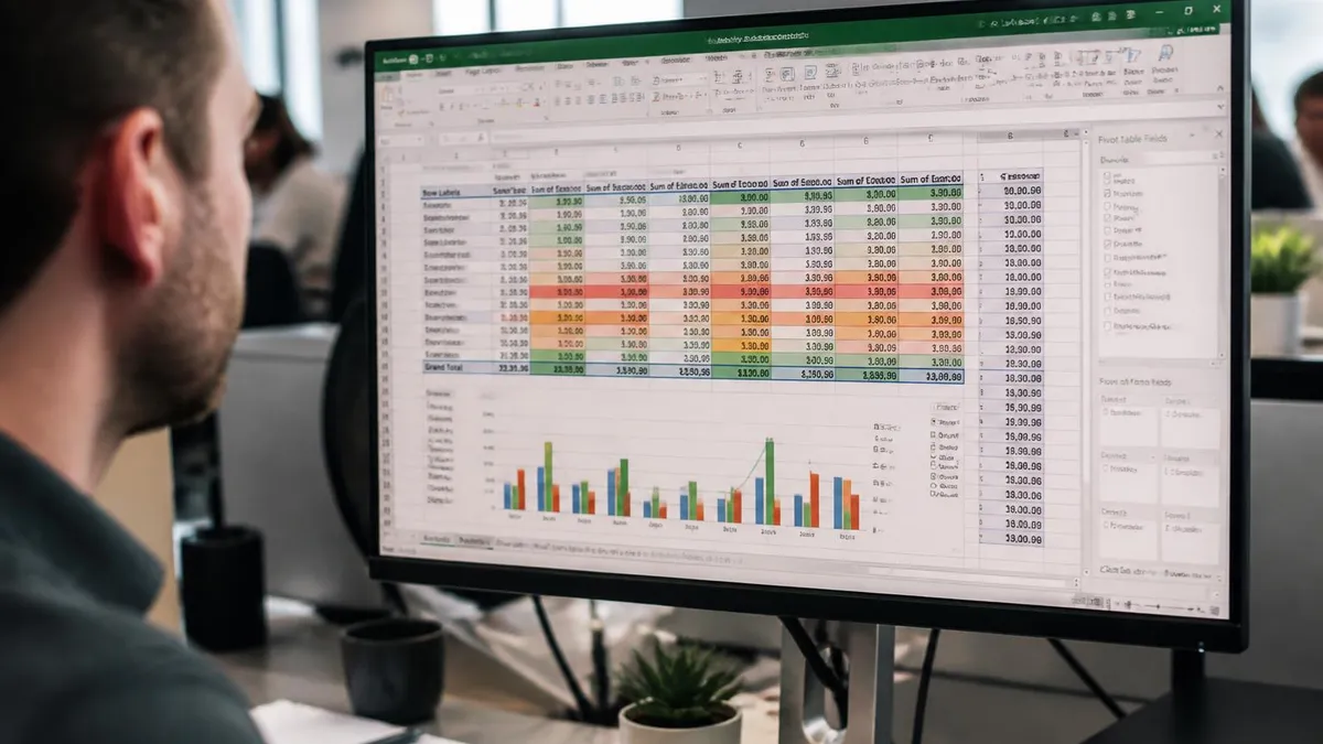
Using too many colors, three-dimensional effects, or excessive chart elements clutters charts and obscures the data message. Pie charts with more than five or six slices become difficult to read. Line charts with more than four series produce visual noise that prevents trend identification. Resisting the temptation to add visual complexity produces clearer charts that communicate more effectively.
Simple two-dimensional chart types consistently produce clearer communication than three-dimensional variants. Reading the chart should be instant rather than requiring careful study to extract the data message from visual complexity.
Working With Multiple Data Series
Multiple data series enable rich comparisons within a single chart. Adding series after the initial chart creation can be done by extending the chart data source or by right-clicking the chart and choosing Select Data. The Select Data dialog allows adding, removing, editing, and reordering data series, as well as adjusting which range provides horizontal axis labels for the chart display.
Combo charts mix different chart types within a single chart, useful when series have different scales or measure different concepts. Right-clicking a data series and choosing Change Series Chart Type opens options to switch that series to a different type such as line while leaving other series as columns. Adding a secondary vertical axis through the same dialog supports series with substantially different value ranges that would otherwise compress on a single shared axis.
Series order affects how the chart reads visually. The first series typically renders behind subsequent series in stacked variants or appears as the leftmost series in clustered variants. Reordering series through Select Data places the most important comparisons in the most prominent positions. Renaming series in the legend through Select Data also improves readability when source headers contain technical column names that would confuse the chart audience.
Data series visibility can be toggled without removing series from the chart. Right-clicking a series and choosing Format Data Series then setting fill to no fill or marker to none hides the series visually while preserving it for potential later display. This technique supports incremental reveal in presentations where speakers want to discuss series one at a time without showing the complete chart immediately.
Trendlines add analytical value to scatter and line charts by showing the overall trajectory of data series. Right-clicking a series and choosing Add Trendline opens options for linear, logarithmic, polynomial, power, exponential, and moving average trendline types. The trendline equation and R-squared value can be displayed on the chart for technical audiences interested in the mathematical fit between trendline and underlying data points.
Excel Chart Creation Checklist
- ✓Identify the data structure and the message before selecting a chart type for the visualization
- ✓Select appropriate data range including headers and category labels for clean automatic labeling
- ✓Choose the simplest chart type that communicates the intended data story without visual clutter
- ✓Add clear chart title that describes what the chart shows in plain language for any reader
- ✓Label axes clearly with units and dimensions visible to viewers without requiring external context
- ✓Use color thoughtfully with attention to contrast and accessibility for diverse audiences
- ✓Remove unnecessary chart elements that distract from the central data message being communicated
- ✓Test chart appearance at presentation viewing distance to verify readability before final delivery
- ✓Save chart formatting as a template if similar charts will be needed across the workbook or future projects
Dynamic Charts That Update Automatically
Static charts work for one-time analysis but business reporting often requires dynamic charts that update as data changes. Excel Tables provide the simplest path to dynamic charts because charts built from Excel Tables automatically extend their data range when new rows are added to the underlying table. Converting a regular range to a table through the Insert Table command produces this dynamic behavior with minimal effort.
Named ranges combined with OFFSET formulas provide more control over dynamic chart data sources but add complexity that most users do not need. The OFFSET formula calculates a dynamic range based on the count of non-empty cells in a reference column, allowing charts to expand and contract based on actual data presence. Power users sometimes prefer this approach for complex dashboards where Excel Table limitations would constrain the design.
PivotCharts represent another dynamic chart approach particularly well suited to dashboards and analytical reports. A PivotChart connects to a PivotTable and inherits all the filtering, grouping, and aggregation capabilities of the underlying PivotTable. Slicers and timeline filters added to the PivotTable apply to the PivotChart automatically, producing interactive visualizations that users can manipulate without modifying the underlying data source.
Slicer integration with PivotCharts produces interactive dashboards that users can filter without modifying source data. Inserting slicers from the PivotChart Analyze tab adds visual filter controls to the worksheet. Clicking slicer buttons filters the underlying PivotTable which automatically updates the connected PivotChart. Multiple slicers can apply simultaneously for combined filtering across several dimensions of the data.
Refresh behavior of dynamic charts depends on data source. Excel Tables update charts automatically as rows are added or modified. External data sources require manual refresh through the Refresh All command on the Data tab or through automated refresh schedules. Power Pivot data models support both manual and scheduled refresh, with refresh frequency aligned to underlying data update patterns in the connected sources.
Saving and Reusing Chart Templates
Custom chart formats can be saved as templates for reuse across workbooks. Right-clicking a finished chart and choosing Save as Template stores the chart formatting in a template file that subsequent charts can apply. The template captures color choices, font sizes, gridline settings, axis formatting, and other visual elements but applies only to charts of the same general type as the original template chart.
Template management through the Insert Chart dialog allows browsing saved templates under the Templates folder. Selecting a template applies all the saved formatting to a newly created chart based on the current selected data. This workflow speeds chart production significantly when many similar charts must be created with consistent branding or formatting across a report or presentation.
Sharing templates across team members requires copying the chart template files between user computers manually or through shared network locations. Excel does not automatically synchronize templates across users or installations. Establishing a shared template library on a network drive or cloud storage solution enables consistent chart formatting across team members without each person needing to recreate templates independently from scratch.
Chart style application from the Chart Design tab provides another reusability mechanism beyond saved templates. Built-in styles offer pre-designed combinations of colors, gridlines, and visual elements that apply with one click. Trying different styles to see how the same data looks under different visual treatments helps identify the most effective presentation without manually formatting individual elements.
Theme files saved as Excel Workbook Themes affect more than just charts but provide comprehensive visual consistency across reports. The theme captures color palettes, fonts, and effect settings that apply to charts, shapes, SmartArt, and even cell formatting throughout the workbook. Sharing theme files across team members synchronizes visual identity across all Excel work products produced by the team.
Excel Charts By the Numbers
Specialty Chart Types
Mix multiple chart types in a single chart to show related data with different scales or different visual conventions across series within the same visualization area. Selecting the right category type matches data structure to visualization convention for clearest communication of the analytical message.
Tiny inline charts that fit within a single cell. Useful for showing trend information alongside data values in dashboard tables without consuming dedicated chart space. Selecting the right category type matches data structure to visualization convention for clearest communication of the analytical message.
Hierarchical visualizations showing nested categories. Treemaps use nested rectangles while sunburst charts use concentric rings for showing organizational structures and category breakdowns. Selecting the right category type matches data structure to visualization convention for clearest communication of the analytical message.
Show how an initial value increases or decreases through a series of contributions to reach a final value. Common for financial bridge analyses showing revenue, costs, and profit components. Selecting the right category type matches data structure to visualization convention for clearest communication of the analytical message.
Troubleshooting Chart Problems
Charts that look wrong often result from improper data selection during initial creation. Selecting too much or too little data, including non-numeric values in numeric columns, or selecting non-contiguous ranges can produce unexpected chart layouts. Redoing the chart with carefully selected data fixes most layout issues. The Select Data dialog allows surgical correction of data ranges without rebuilding the chart from scratch.
Axis scale problems occur when data has very large or very small values mixed together. Excel auto-scaling may compress important variations in the smaller values when larger values dominate the axis range. Manually setting axis minimum and maximum through the Format Axis pane corrects this. Logarithmic axis scales help when data spans multiple orders of magnitude that linear scales cannot display effectively.
Date axis problems occur when Excel interprets date values as text rather than dates. The chart displays dates in source order rather than chronological order, and time intervals between data points may render incorrectly. Converting date columns to genuine date format through cell formatting or the DATEVALUE function resolves this issue. Properly formatted date axes display with intelligent date interval spacing automatically.
Performance issues with charts containing many data series or large data sets benefit from simplification. Reducing data point density by aggregating values weekly or monthly instead of daily reduces chart rendering load. Disabling animation through the chart options improves redraw speed during interactive use. For very large data sets, consider sampling representative data points rather than charting every value.
Compatibility issues arise when charts move between Excel versions or to other spreadsheet applications. Newer chart types such as treemap, sunburst, and waterfall do not display correctly in Excel versions before 2016. Charts copied to PowerPoint may lose formatting if pasted as pictures rather than as linked or embedded chart objects. Testing chart appearance in the destination application before relying on the result prevents surprises during important presentations.
Excel Charts Pros and Cons
- + —
- + —
- + —
- + —
- + —
- − —
- − —
- − —
- − —
- − —
Sample Excel Practice Questions
Try these questions from our free Excel practice tests. The correct answer and an explanation follow each question.
How do you create a dynamic chart title linked to a cell?
- A. Type the cell reference in the title
- B. Click the title, click formula bar, type = and click the cell
- C. Use a macro
- D. Not possible in Excel
Answer: B. Click the title, click formula bar, type = and click the cell
Click the chart title, then use the formula bar to link it to a cell reference.
What is the purpose of error bars in charts?
- A. Highlighting incorrect data
- B. Displaying variability or uncertainty of data points
- C. Showing when data exceeds boundaries
- D. Indicating formula errors
Answer: B. Displaying variability or uncertainty of data points
Error bars represent variability, uncertainty, or margin of error in data.
What chart type is best for showing trends over continuous time?
- A. Pie chart
- B. Line chart
- C. Treemap
- D. Doughnut chart
Answer: B. Line chart
Line charts connect data points across time intervals to show trends.
New records were added to the source table of a PivotChart, but the chart has not changed. What should you do?
- A. Create a new PivotChart
- B. Click Refresh on the PivotChart Analyze tab
- C. Change the chart type
- D. Reapply the chart style
Answer: B. Click Refresh on the PivotChart Analyze tab
PivotCharts do not update until the PivotTable cache is refreshed.
Take the full Excel practice test
📊 How do you create a chart in Excel?
Select the data including its headers, then go to Insert > Recommended Charts and pick a preview, or choose a type from the Charts group. Excel uses the headers and row labels to build the axis labels and legend automatically.
START EXCEL PRACTICE TEST⌨️ What is the fastest keyboard shortcut to insert a chart in Excel?
On Windows, select the data and press Alt+F1 to insert the default chart type embedded on the current sheet. Pressing F11 instead creates the default chart on its own separate chart sheet.
START EXCEL PRACTICE TEST🔄 How do you swap rows and columns in an Excel chart?
Click the chart, open the Chart Design tab and select Switch Row/Column. This swaps which data appears on the horizontal axis and which appears as the legend series, without changing the worksheet data.
START EXCEL PRACTICE TEST🥧 When should you use a pie chart in Excel?
Use a pie chart when you have a single data series whose values add up to a meaningful whole. Each slice is shown as a percentage of the total, so it reads best with only a handful of categories and no negative or zero values.
START EXCEL PRACTICE TEST📈 What is the difference between a line chart and a scatter chart in Excel?
A line chart spaces categories evenly along the horizontal axis, which suits dates and time periods. A scatter (XY) chart plots numeric values on both axes, so it is the right choice for showing the relationship between two numeric variables.
START EXCEL PRACTICE TEST🔀 How do you make a combo chart with a secondary axis in Excel?
Select the chart, go to Chart Design > Change Chart Type and choose Combo. Assign a chart type to each series, such as clustered column plus line, and tick Secondary Axis for the series whose scale differs from the rest.
START EXCEL PRACTICE TEST🧩 What are the Chart Elements, Chart Styles and Chart Filters buttons?
In Excel for Windows, clicking a chart shows three buttons beside it. Chart Elements (the plus sign) adds or removes titles, data labels, gridlines and the legend, Chart Styles changes the style and colors, and Chart Filters hides series or categories.
START EXCEL PRACTICE TEST🔗 How do you link an Excel chart title to a cell?
Click the chart title, click in the formula bar, type an equals sign and then click the cell that holds the title text, and press Enter. The title now updates automatically whenever the cell value changes.
START EXCEL PRACTICE TEST📋 How do you make an Excel chart update automatically when you add new data?
Convert the source range to an Excel Table with Insert > Table or Ctrl+T before you build the chart. A chart built on a Table expands to include new rows added to the bottom, so you do not have to edit the data range by hand.
START EXCEL PRACTICE TEST💾 How do you save and reuse a chart format as a template?
Right-click a finished chart and choose Save as Template, which saves it as a .crtx file. To reuse it, open Insert > Recommended Charts, go to All Charts > Templates and pick your saved template so new charts get the same formatting.
START EXCEL PRACTICE TESTExcel Questions and Answers
Official Resources
- Microsoft Support: Create a chart from start to finish — Microsoft's own walkthrough for inserting, formatting and editing charts in Excel for Windows, Mac and the web.
- Microsoft Support: Available chart types in Office — the official reference describing every Excel chart type and its sub-types, from column and pie to treemap and waterfall.
- Microsoft Learn: MOS Excel Associate (Microsoft 365 Apps) — the official certification page listing the skills measured, including creating and modifying charts.
Written and edited by Nathan Beja, founder of Practice Test Geeks, with AI assistance. Exam facts are checked against the official sources linked below. Editorial policy
Sources & references
Exam facts on this page (fees, format, dates, passing scores) are checked against these official sources; the date is our last check. Editorial policy
- learn.microsoft.com — Retake policy, test delivery, time limit, eligibility · verified Oct 2026
- certiport.pearsonvue.com — Exam format, score validity, passing score, score release, exam information · verified Oct 2026