
Microsoft Excel Tutorial: Master Spreadsheets From Beginner to Advanced
Complete microsoft excel tutorial covering VLOOKUP, drop-down lists, merging cells, freezing rows, and advanced formulas. Practice with free quizzes. 🟢

A solid microsoft excel tutorial is the single fastest way to transform raw data into actionable insights, and millions of professionals worldwide rely on Excel every single day to manage budgets, analyze sales figures, build financial models, and automate repetitive tasks. Whether you are brand new to spreadsheets or looking to sharpen skills you have been using for years, understanding Excel from the ground up will unlock career opportunities and save you dozens of hours each week. This guide walks through every core feature methodically, so even a complete beginner can follow along step by step.
Excel is part of the Microsoft 365 suite, and its capabilities extend far beyond simple arithmetic. Functions like VLOOKUP excel power users need for data lookups, pivot tables for instant summaries, and conditional formatting for visual analysis — these tools turn a blank grid into a sophisticated reporting engine. The program is used in virtually every industry: finance teams build valuation models, marketers track campaign metrics, HR departments manage headcount spreadsheets, and logistics planners optimize supply chains, all inside the same familiar interface.
Understanding how to create a drop down list in Excel, for example, can prevent data-entry errors across an entire department. A validated list ensures that employees select from a predefined set of choices — product categories, status labels, regional codes — instead of typing freeform text that breaks formulas downstream. Small workflow improvements like this compound rapidly, and mastering twenty or thirty such features can realistically double the speed at which you complete routine tasks at the office.
Learning how to merge cells in Excel is another foundational skill that shapes the visual clarity of every report you produce. Merging allows you to create clean, professional-looking headers that span multiple columns, giving your spreadsheets the polished look expected in boardroom presentations and client-facing deliverables. Once you understand when merging helps versus when it hinders sorting and filtering, you will make better layout decisions from the outset rather than reformatting endlessly.
Similarly, knowing how to freeze a row in Excel means you can scroll through thousands of records without ever losing track of which column holds which data field. Frozen panes lock your header row — or any row and column combination — in place while the rest of the sheet scrolls freely. This tiny feature prevents misreading data in large datasets, a mistake that can cause costly analytical errors when reports are built on mislabeled figures.
The institute of creative excellence in data visualization often comes down to mastering Excel charts: bar charts for comparisons, line charts for trends over time, scatter plots for correlations, and waterfall charts for financial bridges. Each chart type tells a different story, and choosing the right one communicates your findings instantly without requiring the reader to interpret a dense table of numbers. Excel's chart customization tools let you match company brand colors, add data labels, and insert trendlines in minutes.
By the end of this tutorial, you will know how to navigate the Excel interface with confidence, build formulas and functions from scratch, manage large datasets efficiently, and create polished reports that impress colleagues and clients. Each section below targets a specific skill area, so you can jump directly to the topic most relevant to your current project or study the full guide from beginning to end for comprehensive mastery.
Free Excel Study Tools
Interactive Excel resources on PracticeTestGeeks, free to start:
- Excel practice test — 500+ questions with instant scoring and answer explanations
- Excel flashcards — review key terms and concepts card by card
- Excel study guide — topic-by-topic overview of what the exam covers
- Excel cheat sheet — one-page printable summary for last-minute review
Microsoft Excel by the Numbers

How to Get Started: Excel Learning Roadmap
Learn the Interface
Master Basic Formulas
Work with Data Tools
Understand Lookup Functions
Build Pivot Tables & Charts
Automate with Macros & Power Query
Once you understand Excel's layout, the next priority is building a working knowledge of formulas and functions — the engine that makes everything else possible. Formulas always begin with an equals sign, followed by a function name, and then the arguments in parentheses. For example, =SUM(A1:A10) adds up all values from cell A1 through A10. Mastering this basic syntax unlocks hundreds of built-in functions that handle everything from rounding numbers to extracting words from text strings and calculating loan repayments.
Absolute versus relative cell references is one of the most important distinctions to understand early. When you write =A1*B1 and copy it down a column, Excel automatically adjusts both references to A2*B2, A3*B3, and so on — that is relative referencing. But if your formula needs to always refer to a specific cell, such as a tax rate in cell B1, you lock it with a dollar sign: =A2*$B$1. Understanding this distinction prevents one of the most common formula errors beginners make.
Logical functions like IF, AND, OR, and NOT let you build decision-making logic directly into cells. A simple =IF(C2>1000,"Bonus","No Bonus") formula, for instance, automatically labels employees who exceeded a sales threshold without any manual review. Nested IF statements handle multiple conditions, though Excel 2019 and Microsoft 365 users are better served by the newer IFS function, which reads more cleanly and supports up to 127 conditions in a single formula without convoluted nesting.
Text functions are invaluable when working with data imported from databases or other systems. TRIM removes extra spaces that cause lookups to fail silently. CONCATENATE (or the modern & operator and CONCAT function) joins text from multiple cells into a single string — useful for combining first and last name columns, building email addresses, or constructing dynamic report titles. LEFT, RIGHT, and MID extract specific portions of text, while FIND and SEARCH locate the position of a character so you can parse data intelligently.
Date and time functions deserve their own attention because date arithmetic confuses many beginners. Excel stores dates as serial numbers — January 1, 1900 is day 1, and each subsequent day increments by one. This means you can subtract two dates to find the number of days between them: =B2-A2. The DATEDIF function calculates the difference in years, months, or days and is commonly used in HR spreadsheets to compute employee tenure or age from a birthdate.
Financial functions are where Excel truly earns its reputation. PMT calculates monthly loan or mortgage payments given a principal amount, interest rate, and number of periods. NPV and IRR evaluate investment projects by discounting future cash flows back to present value. These functions are the reason finance professionals who master a comprehensive microsoft excel tutorial command premium salaries — the ability to model cash flows quickly and accurately is a rare and valued skill in corporate environments everywhere.
Error-handling functions like IFERROR and IFNA make your spreadsheets more strong. Instead of displaying unsightly #N/A or #DIV/0! errors to end users, you wrap your formula: =IFERROR(VLOOKUP(A2,Table1,2,0),"Not Found"). The formula still performs the lookup, but if it fails for any reason, it displays the friendly fallback text you specified. Professional dashboards always include error handling so that incomplete data does not break the entire report or cause confusion among non-technical viewers.
Microsoft Excel Practice Test Questions
Prepare for the Microsoft Excel exam with our free practice test modules. Each quiz covers key topics to help you pass on your first try.
Microsoft Excel Excel Basic and Advance
Microsoft Excel Exam Questions covering Excel Basic and Advance. Master Microsoft Excel Test concepts for certification prep.
Microsoft Excel Excel Formulas
Free Microsoft Excel Practice Test featuring Excel Formulas. Improve your Microsoft Excel Exam score with mock test prep.
Microsoft Excel Excel Functions
Microsoft Excel Mock Exam on Excel Functions. Microsoft Excel Study Guide questions to pass on your first try.
Microsoft Excel Excel MCQ
Microsoft Excel Test Prep for Excel MCQ. Practice Microsoft Excel Quiz questions and boost your score.
Microsoft Excel Excel
Microsoft Excel Questions and Answers on Excel. Free Microsoft Excel practice for exam readiness.
Microsoft Excel Excel Trivia
Microsoft Excel Mock Test covering Excel Trivia. Online Microsoft Excel Test practice with instant feedback.
Microsoft Excel Advanced Data Analysis Tools
Free Microsoft Excel Quiz on Advanced Data Analysis Tools. Microsoft Excel Exam prep questions with detailed explanations.
Microsoft Excel Advanced Formula and Macro...
Microsoft Excel Practice Questions for Advanced Formula and Macro Creation. Build confidence for your Microsoft Excel certification exam.
Microsoft Excel Advanced Formulas and Macros
Microsoft Excel Test Online for Advanced Formulas and Macros. Free practice with instant results and feedback.
Microsoft Excel Basic and Advance Question...
Microsoft Excel Study Material on Basic and Advance Questions and Answers. Prepare effectively with real exam-style questions.
Microsoft Excel Creating and Managing Charts
Free Microsoft Excel Test covering Creating and Managing Charts. Practice and track your Microsoft Excel exam readiness.
Microsoft Excel Data Visualization with Ch...
Microsoft Excel Exam Questions covering Data Visualization with Charts. Master Microsoft Excel Test concepts for certification prep.
Microsoft Excel Formulas and Functions
Free Microsoft Excel Practice Test featuring Formulas and Functions. Improve your Microsoft Excel Exam score with mock test prep.
Microsoft Excel Formulas and Functions App...
Microsoft Excel Mock Exam on Formulas and Functions Application. Microsoft Excel Study Guide questions to pass on your first try.
Microsoft Excel Formulas Questions and Ans...
Microsoft Excel Test Prep for Formulas Questions and Answers. Practice Microsoft Excel Quiz questions and boost your score.
Microsoft Excel Functions Questions and An...
Microsoft Excel Questions and Answers on Functions Questions and Answers. Free Microsoft Excel practice for exam readiness.
Microsoft Excel Managing Data Cells and Ra...
Microsoft Excel Mock Test covering Managing Data Cells and Ranges. Online Microsoft Excel Test practice with instant feedback.
Microsoft Excel Managing Tables and Data
Free Microsoft Excel Quiz on Managing Tables and Data. Microsoft Excel Exam prep questions with detailed explanations.
Microsoft Excel Managing Tables and Table ...
Microsoft Excel Practice Questions for Managing Tables and Table Data. Build confidence for your Microsoft Excel certification exam.
Microsoft Excel Managing Worksheets and Wo...
Microsoft Excel Test Online for Managing Worksheets and Workbooks. Free practice with instant results and feedback.
Microsoft Excel MCQ Questions and Answers
Microsoft Excel Study Material on MCQ Questions and Answers. Prepare effectively with real exam-style questions.
Microsoft Excel Questions and Answers
Free Microsoft Excel Test covering Questions and Answers. Practice and track your Microsoft Excel exam readiness.
VLOOKUP Excel: Lookups, Drop-Down Lists & Cell Merging
VLOOKUP stands for Vertical Lookup and searches for a value in the leftmost column of a table, then returns data from a column you specify to the right. The syntax is =VLOOKUP(lookup_value, table_array, col_index_num, [range_lookup]). Setting the last argument to FALSE ensures an exact match, which is what you almost always want in real-world work. For example, =VLOOKUP(E2,A2:C100,3,FALSE) finds the value in E2 within column A and returns the corresponding entry from column C, making it ideal for price lookups, employee records, and product catalogs.
One key limitation of VLOOKUP excel is that it can only look to the right — the lookup column must always be the leftmost column in your table array. When you need to retrieve data from a column to the left of your search column, INDEX-MATCH is the superior alternative. The formula =INDEX(B2:B100,MATCH(E2,C2:C100,0)) achieves the same goal without positional restrictions. Microsoft 365 users can also use XLOOKUP, which is even more flexible: it searches in any direction, handles errors natively, and returns entire arrays rather than a single value.
Excel vs. Google Sheets: Which Should You Learn First?
- +More powerful functions and formula capabilities than Google Sheets
- +Superior charting tools with more customization options
- +Better performance with very large datasets (millions of rows via Power Query)
- +Macros and VBA scripting for advanced automation without third-party tools
- +Industry standard in finance, banking, consulting, and enterprise environments
- +Offline-first: full functionality without an internet connection
- −Requires a paid Microsoft 365 subscription for the latest features
- −Steeper learning curve for beginners compared to Google Sheets
- −Real-time collaboration is less seamless than Google Sheets co-editing
- −Files can become large and slow when overloaded with formulas and data
- −VBA macros can introduce security vulnerabilities if macros from unknown sources are enabled
- −Version differences between Excel 2016, 2019, 2021, and 365 cause formula compatibility issues
Pros and Cons at a Glance
| Pros | Cons |
|---|---|
| More powerful functions and formula capabilities than Google Sheets | Steeper learning curve for beginners compared to Google Sheets |
| Superior charting tools with more customization options | Real-time collaboration is less seamless than Google Sheets co-editing |
| Better performance with very large datasets (millions of rows via Power Query) | Files can become large and slow when overloaded with formulas and data |
| Macros and VBA scripting for advanced automation without third-party tools | VBA macros can introduce security vulnerabilities if macros from unknown sources are enabled |
Essential Excel Skills Checklist for 2026
- ✓Enter and format data using consistent number, date, and text formats across columns
- ✓Use absolute cell references ($A$1) when copying formulas that reference fixed values
- ✓Apply VLOOKUP or XLOOKUP to retrieve data from a separate reference table
- ✓Create a drop-down list using Data Validation to restrict cell input to valid choices
- ✓Merge cells for report headers while using Center Across Selection for functional layouts
- ✓Freeze the top row and leftmost column to navigate large datasets without losing context
- ✓Build a PivotTable from a flat data range and group by date, category, or region
- ✓Use conditional formatting to highlight cells that meet specific criteria automatically
- ✓Write an IF formula with nested logic or use IFS for multiple conditions
- ✓Protect a worksheet with a password to prevent accidental edits to formulas and structure
Ctrl+Shift+Enter for Array Formulas
Before Excel 365 introduced dynamic arrays, complex multi-cell calculations required Ctrl+Shift+Enter instead of just Enter to create array formulas enclosed in curly braces. Even in modern Excel, knowing this shortcut helps you understand legacy workbooks and work in environments where Microsoft 365 is not available. When you see {=SUM(A1:A10*B1:B10)} in a cell, those curly braces indicate an array formula entered with this shortcut.
Charts and data visualization are where Excel transforms from a calculation tool into a communication platform. Before creating any chart, ask yourself what story you are trying to tell: a comparison between categories calls for a bar or column chart, a trend over time needs a line chart, and a part-to-whole relationship is best shown as a pie or doughnut chart. Choosing the wrong chart type can mislead your audience or obscure the very insight you are trying to highlight, so this decision deserves deliberate thought before you click Insert Chart.
To create a chart, select your data range — including headers — and press Alt+F1 to insert a default chart, or navigate to Insert > Charts and choose your preferred type. Excel immediately generates a chart that you can resize, reposition, and format through the Chart Design and Format tabs that appear in the Ribbon. Right-clicking any chart element opens a context menu with granular formatting options: you can change fill colors, add data labels that display exact values, adjust axis scales, and insert a trendline with a single click.
PivotTables are arguably Excel's single most powerful feature for anyone who works with large datasets regularly. To create one, click anywhere inside a flat data table, navigate to Insert > PivotTable, and choose whether to place it in a new or existing worksheet. The PivotTable Field List appears on the right, showing all column headers from your source data. Drag fields into the Rows, Columns, Values, and Filters areas to instantly summarize thousands of records by any combination of dimensions, without writing a single formula.
Slicers and timelines make PivotTables interactive. A slicer is a visual filter button that users can click to show only specific categories, like a particular region or product line. A timeline works the same way but specifically for date fields, allowing users to drag a range selector to filter by month, quarter, or year. These features make PivotTable-based dashboards feel dynamic and professional, enabling non-technical stakeholders to explore data independently without knowing anything about filters or formulas.
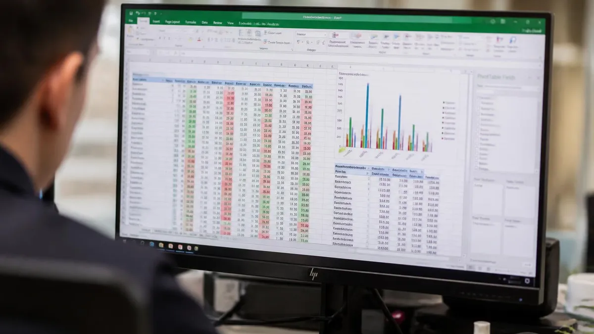
Conditional formatting deserves special attention as both a data analysis and visualization tool. Select a range, go to Home > Conditional Formatting, and choose from options like Color Scales (which gradient-fills cells from red to green based on their values), Data Bars (mini bar charts inside cells), Icon Sets (arrows, traffic lights, stars), or custom rules based on formulas. A common use case is highlighting all cells in a sales column that fall below target in red and those above target in green, giving managers an instant visual summary without reading every number individually.
Sparklines are a lesser-known but extremely useful visualization feature. They are tiny charts embedded directly inside individual cells, typically used to show trends for each row in a table. Select your sparkline data range, go to Insert > Sparklines, and choose Line, Column, or Win/Loss style. Sparklines appear in the cells you specify and update automatically when data changes. They are perfect for dashboards where space is limited but you still want to convey directional trends alongside the actual numbers in adjacent columns.
Power Query, accessed through the Data > Get & Transform Data menu, is the modern way to import and clean data from external sources including CSV files, databases, web pages, and SharePoint lists. Every transformation step you apply — removing blank rows, splitting columns, merging tables, changing data types — is recorded as a step in the Query Editor and can be re-run with a single click whenever new data arrives. This replaces hours of manual data cleaning each reporting cycle with a repeatable, one-click refresh workflow.
Storing numbers as text is one of the most common Excel pitfalls — it causes SUM formulas to return zero and lookups to fail silently. Always check that number columns show right-aligned values (numbers) rather than left-aligned text. If you see a green triangle in cell corners, click the warning icon and choose Convert to Number. Also avoid storing multiple pieces of information in one cell; splitting first name, last name, city, and state into separate columns keeps your data relational and filterable.
Advanced Excel users distinguish themselves by combining multiple features into cohesive workflows rather than using each tool in isolation. A typical financial reporting workflow, for example, might use Power Query to import raw transaction data from an accounting system, a series of calculated columns using structured table formulas to categorize and flag records, a PivotTable to summarize totals by department and month, and a dashboard sheet with charts and slicers for executives. Each component feeds the next, and the entire model refreshes in seconds when the source data updates.
Dynamic array functions introduced in Excel 365 represent a fundamental shift in how formulas work. Functions like FILTER, SORT, UNIQUE, and SEQUENCE return arrays of results that spill automatically into adjacent cells without requiring Ctrl+Shift+Enter. For example, =FILTER(A2:C100,B2:B100="West") returns all rows where the region column contains West, updating instantly when data changes. These spill functions eliminate the need for many helper columns and complex array formulas that were previously required to achieve the same results.
Named ranges and Excel Tables (created with Ctrl+T) make your formulas dramatically more readable and maintainable. Instead of writing =VLOOKUP(E2,$A$2:$C$500,3,FALSE), you can define the range as SalesData and write =VLOOKUP(E2,SalesData,3,FALSE). Excel Tables go further: they expand automatically when you add rows, give columns structured reference names, and enable total rows with dropdown aggregations. Any formula that references a Table column automatically includes new rows, eliminating the need to manually update formula ranges as data grows.
Macro recording and basic VBA programming represent the ceiling of Excel automation capability. To record a macro, go to View > Macros > Record Macro, perform the steps you want to automate, then stop recording. Excel translates your actions into VBA code stored in the workbook. You can then run the macro with a single button click or keyboard shortcut, repeating those exact steps on any dataset in seconds. More advanced users edit the recorded VBA code directly to add conditional logic, loops, and user input dialogs that recording alone cannot capture.
Data validation extends beyond drop-down lists to include whole number ranges, decimal constraints, date boundaries, text length limits, and custom formula-based rules. For example, you might restrict an invoice date column to only accept dates within the current fiscal year, or prevent duplicate entries in an ID column using a COUNTIF-based custom rule. Combined with input messages and error alerts, data validation creates forms that guide users toward correct entries and reject invalid data before it can corrupt your analysis or downstream reports.
For those pursuing Microsoft Office Specialist (MOS) certification or preparing for technical interviews, a structured microsoft excel tutorial practice approach is essential. The MOS Excel Associate exam tests skills across creating and managing workbooks, managing data cells and ranges, creating tables, performing operations with formulas and functions, and managing charts. The Expert exam adds managing workbook options, managing and formatting data, creating advanced formulas and macros, and managing advanced charts and PivotTables. Practice tests that simulate the exam's task-based format are the most effective preparation method available.
The most effective approach combines all three: read the concept, watch it applied, then immediately replicate it yourself on a live spreadsheet. Spaced repetition — revisiting skills at increasing intervals — builds long-term retention far better than cramming all features in a single marathon session.
Building real projects is the most accelerated path to Excel mastery. Rather than working through disconnected exercises, challenge yourself to solve actual problems you face at work or in personal life: build a personal budget tracker, create an inventory management spreadsheet for a small business, model the amortization schedule for a hypothetical mortgage, or analyze a public dataset from a government database. Real projects force you to encounter edge cases, debug formula errors, and make design decisions that tutorials can never fully simulate.
The inner excellence book principle — that mastery comes from deliberate practice focused on specific weaknesses — applies directly to learning Excel. Rather than practicing what you already know well, identify your current weakest area: perhaps it is PivotTables, perhaps it is nested IF formulas, perhaps it is data cleaning with Power Query. Dedicate focused thirty-minute sessions to that specific weakness, deliberately practice it on varied examples, and track your progress. This targeted approach builds competence faster than general review of material you already understand.
Excel keyboard shortcuts deserve dedicated practice because they dramatically reduce the time spent navigating menus. The most valuable shortcuts include Ctrl+C and Ctrl+V for copy and paste, Ctrl+Z for undo, Ctrl+Home and Ctrl+End to jump to the beginning and end of your data, F2 to enter edit mode in a cell, Ctrl+D to fill down, and Ctrl+Shift+L to toggle AutoFilter on and off. Power users who rarely touch the mouse can work two to three times faster than those who navigate exclusively through the Ribbon and right-click menus.
Collaboration features in modern Excel have improved dramatically. Co-authoring allows multiple users to edit the same workbook simultaneously in Excel 365 with changes reflected in near real-time, similar to Google Sheets. Comments and threaded conversations can be attached to specific cells, allowing team members to discuss data points, flag questions, and resolve discrepancies without switching to email or chat. Version history in SharePoint and OneDrive lets you view and restore any previous version of a shared workbook, providing a safety net when accidental overwrites occur.
Data security is increasingly important as workbooks often contain sensitive financial, personnel, or customer information. Excel provides several protection layers: cell-level protection restricts editing of formulas and critical inputs, sheet-level protection prevents structural changes like adding or deleting rows and columns, and workbook-level protection controls who can add, rename, or hide worksheets. Encrypting a workbook with a password (File > Info > Protect Workbook > Encrypt with Password) prevents unauthorized users from opening the file entirely, which is appropriate for documents containing personally identifiable information or proprietary financial data.
Hotels build occupancy models that pull historical booking data, apply seasonal adjustment factors, and project forward revenue at different rate scenarios. Restaurant groups use Excel to track food cost percentages, calculate theoretical versus actual inventory variances, and model menu pricing changes across hundreds of items simultaneously.
As you continue your learning journey, supplement your practice with Excel's built-in Help system (F1) and the official Microsoft support documentation, which includes step-by-step guides for every function and feature. Community forums like MrExcel and the Microsoft Tech Community have archives of thousands of solved problems where you can find answers to specific formula challenges. Most importantly, maintain a personal formula library — a workbook where you save particularly useful formulas, techniques, and template structures — so that solutions you discover once are immediately available the next time you encounter a similar problem.
If you want the full picture, the microsoft excel tutorial guide walks through it step by step.
For a deeper look at this topic, see our guide to microsoft excel tutorial.
Sample Excel Practice Questions
Try these questions from our free Excel practice tests. The correct answer and an explanation follow each question.
How does Advanced Filter differ from AutoFilter?
- A. Advanced Filter is slower
- B. Can extract to another location, use complex AND/OR criteria, find unique records
- C. Only works with Tables
- D. Identical functionality
Answer: B. Can extract to another location, use complex AND/OR criteria, find unique records
Advanced Filter supports complex multi-field AND/OR criteria, copying results elsewhere, and unique records.
A company policy requires that all macros in workbooks must be disabled by default, but users should be notified with a security warning and given the option to enable them if the workbook is from a trusted source. Which Macro Security setting in the Trust Center achieves this balance?
- A. Enable all macros (not recommended)
- B. Disable all macros without notification
- C. Disable all macros with notification
- D. Disable all macros except digitally signed macros
Answer: C. Disable all macros with notification
The 'Disable all macros with notification' setting is the default and most common security level. It prevents macros from running automatically but provides a message bar, allowing the user to enable content on a case-by-case basis.
To compare data from two different worksheets within the same workbook side-by-side, which sequence of commands on the 'View' tab is correct?
- A. Arrange All > Vertical
- B. Split > Arrange All
- C. New Window > Arrange All > Vertical
- D. Freeze Panes > View Side-by-Side
Answer: C. New Window > Arrange All > Vertical
To view two sheets from the same workbook, you first need to open a second window of the current workbook using 'New Window'. Then, you can use 'Arrange All' and select an option like 'Vertical' to display both windows (and thus, different sheets) side-by-side.
How does ROUND differ from TRUNC?
- A. ROUND works with negatives, TRUNC does not
- B. ROUND applies mathematical rounding, TRUNC removes decimals without rounding
- C. They produce identical results
- D. TRUNC is more precise
Answer: B. ROUND applies mathematical rounding, TRUNC removes decimals without rounding
ROUND follows rounding rules (5 rounds up); TRUNC simply cuts off digits.
Excel Questions and Answers

Excel Finance Functions Guide With PMT, NPV, IRR and Loan Models

Excel Merge Tables: The Complete 2026 Guide to Combining Data Across Worksheets

Lock Formulas in Excel: The Complete 2026 Guide to Protecting Cells, Sheets, and Workbook Calculations

Excel Data Analysis Toolpak: Complete Guide to the Analysis ToolPak Add-In

Mail Merge Labels from Excel: The Complete 2026 Guide to Printing Address Labels with Word and Excel
About the Author

Business Consultant & Professional Certification Advisor
Wharton School, University of PennsylvaniaKatherine Lee earned her MBA from the Wharton School at the University of Pennsylvania and holds CPA, PHR, and PMP certifications. With a background spanning corporate finance, human resources, and project management, she has coached professionals preparing for CPA, CMA, PHR/SPHR, PMP, and financial services licensing exams.