DAYS Function in Excel: The Complete Guide to Calculating Date Differences Like a Pro in 2026

The days excel function is one of the most underrated time-saving formulas in the entire spreadsheet toolkit, and once you understand how it works, you will wonder how you ever managed deadlines, aging reports, or project timelines without it. At its core, DAYS returns the number of days between two dates, and it does so with a simple two-argument syntax that even spreadsheet beginners can master in about ten minutes of focused practice on real worksheets.

Microsoft introduced DAYS in Excel 2013, and it has since become a staple in finance, accounting, human resources, logistics, and project management workflows across every industry. Unlike the older DATEDIF function, DAYS is fully documented, fully supported, and behaves predictably across Windows, Mac, and Excel for the web. That consistency matters when you are building templates that other people will open on different machines and different Excel versions.

If you have ever struggled with vlookup excel formulas that pull dates from another sheet only to realize you still need to compute the gap between those dates, DAYS is the natural partner. You can nest it inside IF statements, combine it with TODAY for live aging calculations, or wrap it inside SUMPRODUCT to count overdue invoices across an entire ledger without writing a single line of VBA code or building any helper columns.

This guide walks you through the syntax, the most common business use cases, the pitfalls that trip up new users, and the advanced patterns that senior analysts use every day. You will see examples for accounts receivable aging, employee tenure tracking, contract expiration alerts, and project burndown reports. Each example uses real numbers you can copy directly into your own workbook and adapt to your data within minutes, not hours.

By the end of this article, you will know exactly when to use DAYS, when to reach for NETWORKDAYS instead, and how to handle the edge cases that involve negative results, text-formatted dates, and the famous 1900 leap year bug that Excel inherited from Lotus 1-2-3 decades ago. We will also cover error messages like #VALUE! and #NUM! so you can debug formulas the moment something looks wrong on your dashboard or report.

Whether you are a financial analyst calculating days sales outstanding, an HR specialist tracking probation periods, or a project manager monitoring milestone slippage, this guide gives you the practical knowledge to use DAYS with total confidence. Bookmark this page, keep it open in another tab as you work, and treat the examples as a personal reference library that grows more useful every time you return to it for a new spreadsheet challenge.

Understanding how DAYS works under the hood will save you hours of debugging time when formulas behave unexpectedly. Excel stores every date as a sequential serial number, starting with January 1, 1900 as serial number 1 and incrementing by one for each subsequent day. When you type a date like 5/21/2026 into a cell, Excel quietly converts it to the serial number 46163 and displays it in whatever date format your locale prefers, which can vary between US and European conventions.

The DAYS function takes the two serial numbers, subtracts start_date from end_date, and returns the difference as a whole integer. That is it. No magic, no time zone conversions, no calendar arithmetic. This simplicity is precisely why DAYS is so reliable across versions, platforms, and locales. If you have ever needed to use vlookup excel to pull a date from a lookup table, you can wrap that VLOOKUP directly inside DAYS without any intermediate steps or helper columns to clutter your workbook.

Here is a concrete example. Imagine you have an invoice issued on March 15, 2026 in cell A2 and a payment received date of April 28, 2026 in cell B2. The formula =DAYS(B2,A2) returns 44, telling you the customer took 44 days to pay. That number flows directly into days sales outstanding calculations, aging buckets, and collection performance dashboards that finance teams review every single Monday morning across thousands of companies worldwide.

One subtle behavior worth memorizing is how DAYS handles text-formatted dates. If you pass a string like "2026-05-21" enclosed in double quotes, Excel attempts to parse it using your system locale settings. This usually works on US systems but can fail unpredictably on machines configured for European date formats where day comes before month. The safest practice is always to use the DATE function or direct cell references that contain real date values, never text strings that might be misinterpreted on different computers.

DAYS also gracefully handles dates that include time components. If your end_date cell contains 5/21/2026 3:45 PM and your start_date contains 5/20/2026 8:00 AM, DAYS still returns 1, because it ignores the time portion entirely and looks only at the integer part of the serial number. If you need fractional days that account for hours and minutes, you would simply subtract the cells directly using the minus operator and format the result as a regular number instead.

Negative results are perfectly valid and intentionally supported by the function. If you reverse the arguments accidentally, the formula returns a negative integer rather than throwing an error. Some analysts deliberately exploit this behavior to build countdown formulas where a negative number signals an overdue task and a positive number signals time remaining. Conditional formatting on the sign of the result creates instant visual cues that highlight problems before they grow into bigger issues for the team.

The real power of DAYS becomes clear when you see it applied to actual business problems. Let us walk through five concrete scenarios where this function quietly drives critical reporting and decision making across departments. Each example uses simple cell references and minimal nesting so you can adapt the pattern to your own workbook in under five minutes of focused effort, even if you have only basic spreadsheet experience under your belt today.

Accounts receivable aging is the classic use case. In column A you have invoice numbers, column B has issue dates, and column C calculates =DAYS(TODAY(),B2). The result is the number of days the invoice has been outstanding. Add a fourth column with nested IF statements that bucket the result into 0-30, 31-60, 61-90, and 90-plus categories. Finance teams use this exact pattern to generate weekly collection priority lists for the credit team.

Employee tenure tracking is another natural fit. Human resources teams maintain rosters with hire dates in one column and use =DAYS(TODAY(),hire_date_cell)/365.25 to compute years of service for anniversary recognition, vacation accrual, and benefits eligibility. The 365.25 divisor accounts for leap years and produces a result accurate to within a day or two over typical employment durations of five to fifteen years at most organizations across the country.

Contract expiration alerts work in reverse direction. Place renewal dates in column B and use =DAYS(B2,TODAY()) to compute days until expiration. Wrap the formula in IF logic that displays warnings like "EXPIRES SOON" when the result drops below 30 or "EXPIRED" when it goes negative. Legal and procurement teams rely on this pattern to avoid auto-renewal surprises and missed negotiation windows that cost thousands in unnecessary fees.

Project milestone variance is calculated by comparing planned and actual completion dates side by side. Column B holds the planned date, column C holds the actual date, and column D contains =DAYS(C2,B2). A positive result means the milestone slipped past its plan, while a negative result means the team delivered early. Project managers roll these variances up to portfolio level dashboards that executives review during monthly steering committee meetings.

Customer churn analysis uses DAYS to measure days since last purchase. Marketing teams build segmentation cohorts based on =DAYS(TODAY(),last_order_date) and trigger re-engagement campaigns when customers cross 60, 90, or 180 day thresholds. The same pattern works for subscription renewal predictions, content engagement scoring, and lifecycle stage classification in any customer relationship management system that exports cleanly to Excel format for further analysis.

Even a simple function like DAYS can throw errors that stop your workflow cold if you do not know what they mean. The three most common error messages are #VALUE!, #NUM!, and #NAME?, and each has a specific root cause that you can diagnose in under a minute once you recognize the pattern. Let us go through each one in detail so you can fix formulas quickly the next time something looks wrong on your dashboard during a critical reporting deadline at the end of the quarter.

#VALUE! appears when one of your arguments is text that Excel cannot interpret as a date. The fix is to check the source cells for stray characters, leading apostrophes, or values that look like dates but are actually formatted as text. Use the ISNUMBER function to test whether each cell holds a real date serial number, since dates are technically numbers under the hood. If ISNUMBER returns FALSE, you have a text value that needs conversion before the DAYS function can process it correctly.

#NUM! errors are rare with DAYS but can occur if you pass extremely large or negative serial numbers that fall outside the valid date range of January 1, 1900 to December 31, 9999. This usually happens when a calculation upstream produces an unexpected result that flows into your DAYS formula as input. Trace the source by clicking Trace Precedents in the Formula Auditing ribbon group to identify where the bad number originated in your workbook before attempting any other troubleshooting steps.

#NAME? means you misspelled the function name or you are working in a version older than Excel 2013 where DAYS does not exist yet. The fix for the spelling issue is obvious, but the version issue requires either upgrading Excel or falling back to simple subtraction like =B2-A2 with the result cell formatted as General to display the day count. Older versions also support DATEDIF as a workaround, although the argument order is reversed from DAYS as we discussed in earlier sections of this guide.

Locale issues cause subtle bugs that do not throw errors but produce wrong results silently. If your machine is set to British English with day-month-year format and a colleague sends a workbook saved on a US machine with month-day-year format, dates near the start of a month can be reinterpreted incorrectly. For example, 3/4/2026 could mean March 4 or April 3 depending on locale. Always use DATE function syntax or ISO format YYYY-MM-DD when sharing across regions to prevent this entire category of subtle bug.

Time component contamination is another silent killer. If your start_date cell secretly contains a time portion like 8:30 AM, DAYS still works correctly because it floors the serial number. But if you accidentally use subtraction instead of DAYS, you get a fractional result that displays as an integer in number format yet behaves like a decimal in further math. Always prefer DAYS over subtraction when integer day counts matter for your downstream calculations and aging reports.

Finally, watch for circular references when combining DAYS with TODAY in cells that themselves feed into date calculations elsewhere in your workbook. Excel will warn you with a status bar message, but the warning is easy to miss when you are working quickly. A circular reference involving TODAY can cause your entire workbook to recalculate slowly or produce inconsistent results between sessions, especially when you have iterative calculation enabled in your Excel options dialog box for some other reason entirely.

Now that you understand the syntax, use cases, and common pitfalls, let us cover the advanced patterns that separate competent Excel users from true power users in the workplace. These techniques combine DAYS with other functions to solve problems that would otherwise require macros, Power Query transformations, or external scripts. Master these five patterns and you will handle 95 percent of date arithmetic challenges that come across your desk during a typical business week at any modern company today.

Pattern one is the conditional aging bucket. Wrap DAYS inside a nested IF or IFS statement to classify invoices into aging categories automatically. For example, =IFS(DAYS(TODAY(),B2)<=30,"Current",DAYS(TODAY(),B2)<=60,"31-60 Days",DAYS(TODAY(),B2)<=90,"61-90 Days",TRUE,"Over 90 Days") produces clean text labels that pivot tables can group and summarize without any helper columns or VBA code cluttering up your otherwise clean and presentable workbook structure.

Pattern two combines DAYS with SUMPRODUCT to count rows meeting date-based criteria across an entire range. The formula =SUMPRODUCT((DAYS(TODAY(),A2:A100)>60)*1) counts how many dates in the range are more than 60 days old. This is faster than COUNTIFS for complex multi-condition date filters and works in every Excel version from 2013 forward without requiring you to commit array formulas with Control plus Shift plus Enter keyboard combinations like the old days.

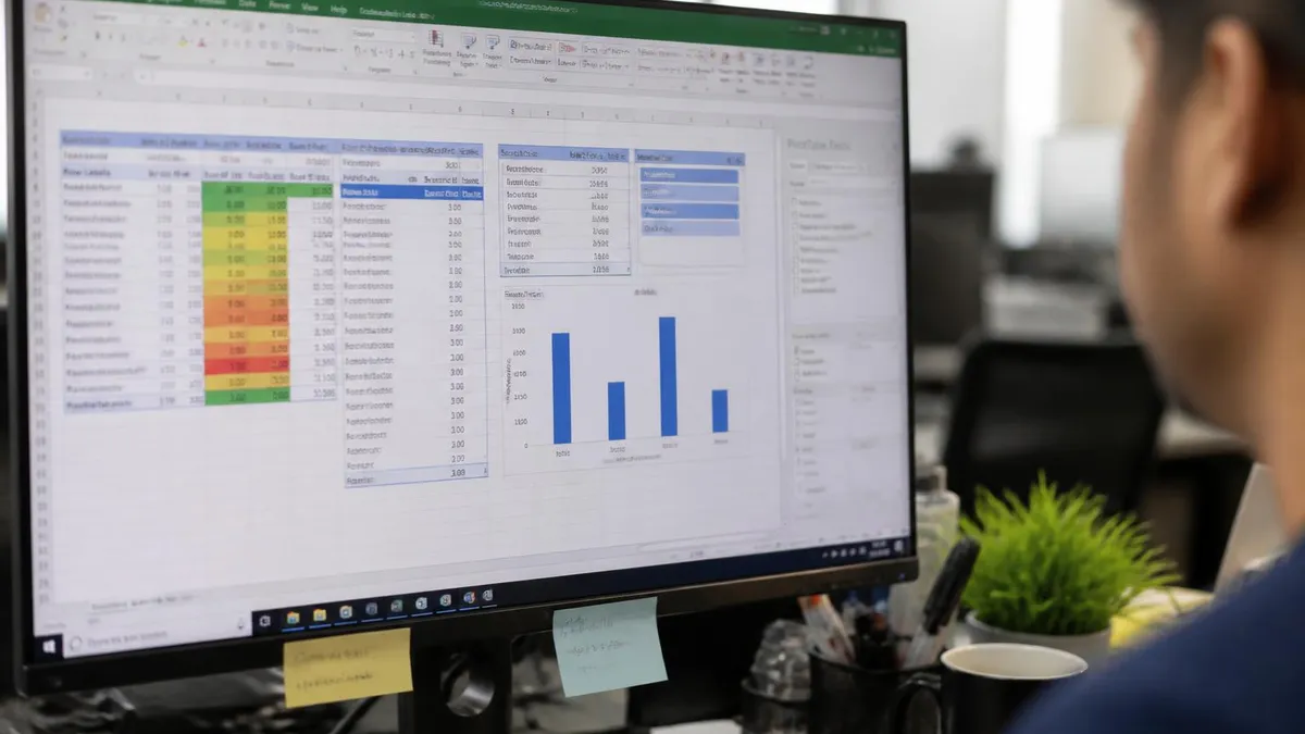
Pattern three integrates DAYS with conditional formatting to create visual heat maps. Select your aging column, open Conditional Formatting, choose Color Scales, and Excel will automatically shade newer invoices green and older invoices red. Combine this with data bars in an adjacent column for double visual encoding that makes overdue items leap off the page during stakeholder reviews. Executives appreciate visual cues that let them grasp the state of the business in seconds rather than minutes of staring at numbers.

Pattern four uses DAYS inside dynamic array formulas with the FILTER function. The formula =FILTER(A2:C100,DAYS(TODAY(),B2:B100)>90) returns only rows where the date in column B is more than 90 days old, automatically spilling the results into adjacent cells. This is the modern replacement for AutoFilter when you need a permanent filtered view that updates as source data changes throughout the day during active reporting cycles or month-end close processes at finance departments.

Pattern five wraps DAYS in IFERROR for production-grade robustness. The formula =IFERROR(DAYS(B2,A2),"") returns an empty string when either date is missing or invalid, keeping your dashboard clean and free of unsightly error indicators. Always add IFERROR wrappers to formulas that will be reviewed by executives or external auditors, since visible errors undermine confidence in your work even when the underlying logic is completely correct and the missing inputs are entirely expected for new records.

Finally, remember that DAYS is just one tool in a much larger date arithmetic toolkit. Pair it with EOMONTH for month-end calculations, EDATE for adding months to a date, WEEKDAY for day-of-week analysis, and WORKDAY for project scheduling. The combination of these functions covers virtually every date computation a business analyst will encounter during a career spanning decades. Bookmark the Excel function reference and revisit it whenever a new requirement lands on your desk that involves date math of any complexity.