
How to Number Rows in Excel: ROW, SEQUENCE & Fill Methods 2026 September
📚 Number rows in Excel the right way. ROW(), SEQUENCE, fill handle, SUBTOTAL for filtered data, Power Query index — pick the method that fits.

Numbering rows in Excel sounds like a two-second job. Drag a corner, done. But the moment you sort, filter, or insert a new row, that tidy column of 1, 2, 3 falls apart. And then you're stuck wondering whether to redo it by hand or hunt for the right formula.
There's more than one way to do this. The fill handle works fine for static lists. The ROW function fixes itself after you delete a row. SEQUENCE (Excel 365) spits out a whole array in one cell. Power Query adds an index column that updates on refresh. Each one solves a different headache.
This guide walks through every method — when to use it, how to type it, and what breaks it. By the end you'll know which approach fits your spreadsheet, whether you're labeling 30 invoice lines or numbering 50,000 rows of survey data. Quick heads-up: if you skip past the basics, jump straight to the SUBTOTAL trick. That's the one people miss.
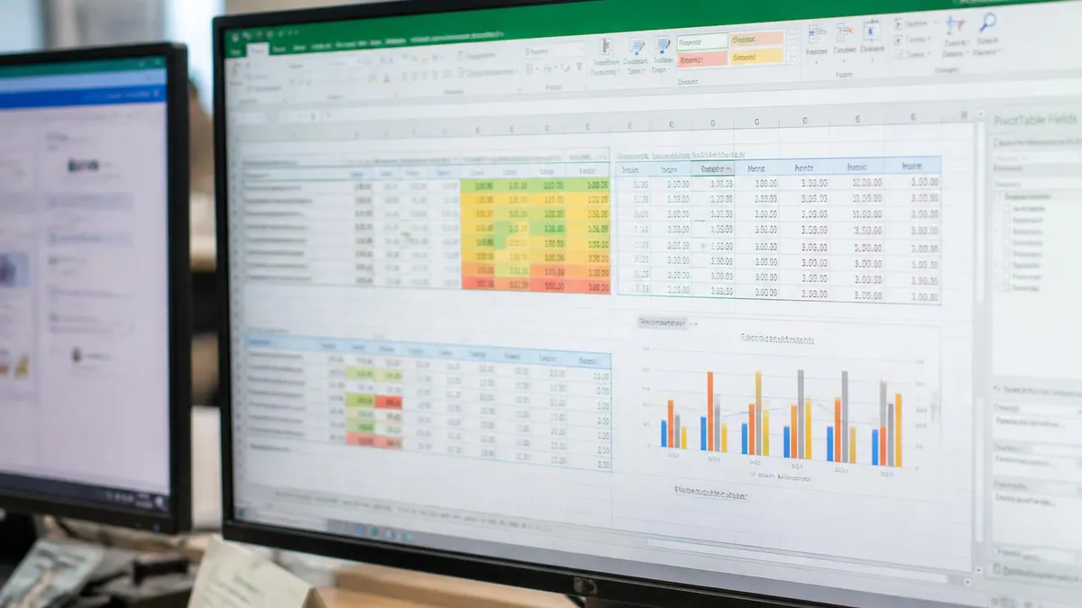
Numbering Methods at a Glance
Before you pick a method, think about what your data actually does. A static price list? Fill handle is perfect. A filtered table where you want visible rows numbered 1, 2, 3? You'll need SUBTOTAL. Got Excel 365 or Excel for the web? SEQUENCE is faster than anything else.
Here's the thing nobody mentions in tutorials — most people learn one method and force it onto every situation. That's why their spreadsheets break. The fill handle is great until you sort. ROW formulas survive sorting but die when you insert a blank row in the middle. SEQUENCE handles arrays beautifully, yet won't work in Excel 2019 or earlier.
A quick note on Excel versions before we dive in. Excel 2010, 2013, and 2016 give you the fill handle, Series Fill, ROW(), and SUBTOTAL — that's it. Excel 2019 added a few new functions but still no SEQUENCE. Excel 2021 brought dynamic arrays and SEQUENCE became available. Excel 365 (the subscription version) gets everything plus regular updates with new functions. Check yours by going to File > Account > About Excel. The version number tells you what's possible.
If you're on Excel for Mac, all the same methods work — keyboard shortcuts differ slightly (use Cmd instead of Ctrl), and the Fill menu sits in a different spot under Edit > Fill. Excel for the web (the free browser version) supports everything except Power Query.
Static list, won't change? Fill handle or Series Fill.
Data gets sorted or rows deleted? Use =ROW()-1.
Working with filtered data? Use =SUBTOTAL(3,B$2:B2).
Have Excel 365? =SEQUENCE(100) — one cell, done.
Big data / refreshable query? Power Query Index Column.
The fill handle is that tiny green square at the bottom-right corner of a selected cell. Click it, drag, and Excel fills the pattern. To number rows the manual way: type 1 in your first row, 2 below it. Select both cells. Grab the fill handle. Drag down as far as you need. Excel reads the pattern and continues the sequence.
Faster trick — double-click instead of drag. If your adjacent column already has data, double-clicking the fill handle auto-fills down to the last row of that neighboring column. Saves you from manually scrolling through 8,000 rows.
But here's where it falls apart. Sort the table? The numbers stay attached to whatever cell they were in, so row 47 might now show 12. Filter out half the rows? You'll see 1, 4, 7, 13, 22 — gaps everywhere. Delete row 15? Now you've got 14, 16, 17 with a missing slot. Fill handle gives you static numbers. They look right at the moment you make them, then they stop being right.
Fill Handle vs Series Fill
Type 1 and 2, select both, drag the green square down. Fast for small ranges. Double-click to auto-fill to the bottom of adjacent column data.
Numbers are static. Sort, filter, or delete rows and you'll see gaps, duplicates, or wrong sequences. Re-do every time data changes.
Home > Editing > Fill > Series. Set step value and stop value. Excel fills 50,000 rows in one click. No dragging required.
Fill handle for under 100 rows of static data. Series Fill for bulk numbering thousands of rows at once. Neither survives sorting.

The Series Fill dialog is the fill handle's grown-up sibling. It gives you precise control: start value, step, stop value. Way better than dragging when you need a specific range.
Click in your first cell. Go to Home > Editing > Fill > Series. A dialog pops up. Pick Columns for vertical numbering. Set Step value to 1 (or 5 if you want 5, 10, 15). Set Stop value to your last number — say, 5000. Hit OK. Excel populates the column instantly. No dragging, no scrolling.
This is genuinely useful when you've got thousands of rows. Try dragging the fill handle through 50,000 cells. You'll be there a while. The Series dialog does it in one click.
Now we're getting into formula territory — which means numbers that actually stay correct.
The ROW() function returns the row number of the cell it sits in. So if you type =ROW() into cell A2, it spits out 2. Not what you want for a numbered list starting at 1. The fix is simple math: subtract the header offset.
In A2, type =ROW()-1. Now A2 shows 1, A3 shows 2, A4 shows 3. Copy that formula all the way down. If you delete row 50, everything below shifts up and renumbers automatically. Insert a row in the middle? Same deal — the numbers self-correct as long as you copy the formula into the new cell.
Why this beats the fill handle: ROW is dynamic. The cell knows where it lives. Move it, copy it, sort it — the formula re-evaluates from scratch every time. For most everyday numbering jobs, this is the right answer.
ROW Function Patterns
Most common pattern. In A2 (with header in A1): =ROW()-1
Returns 1, 2, 3... down the column. Survives row deletion — formulas re-evaluate after the shift. Doesn't survive filtering — hidden rows still count.
So far so good — until you filter your data. Apply a filter to hide half the rows and your ROW()-1 formulas keep showing their original numbers. You'll see visible rows labeled 3, 7, 14, 22 instead of 1, 2, 3, 4. Looks broken because, well, it kind of is.
Enter SUBTOTAL. It's a function most people use for sums and averages, but it has a hidden skill: it ignores hidden rows.
In A2, type: =SUBTOTAL(3,B$2:B2). Function number 3 means COUNTA — count non-empty cells. The trick is the absolute reference B$2 as the anchor and a relative B2 as the endpoint. As you drag the formula down, the range expands. Excel counts how many visible non-empty cells exist from B2 down to the current row.
Filter the data — boom, visible rows renumber to 1, 2, 3 instantly. Remove the filter, they go back to matching the full list. This is the formula advanced users reach for when they need numbering that respects filters.
Forgetting the absolute anchor breaks the whole formula. =SUBTOTAL(3,B2:B2) with no $ signs will just return 1 for every row — because the range never expands.
Correct version: =SUBTOTAL(3,B$2:B2). The B$2 locks the starting point. As you fill down, only the end of the range grows. That's how the count increments.
SEQUENCE is the new kid. It only exists in Excel 365, Excel for the web, and Excel 2021 onward. If you've got one of those — congrats, this is the cleanest method.
Click into cell A2 and type =SEQUENCE(100). Press Enter. Excel spills 100 numbers down the column — 1, 2, 3, all the way to 100. One formula, no dragging, no copying. The result is a dynamic array; you can't delete individual cells in the spill range without deleting the whole thing.
Need to start at a different number? =SEQUENCE(100,1,5,2) gives you 100 rows, 1 column, starting at 5, stepping by 2. So 5, 7, 9, 11... up to 203. Want a 2D grid? =SEQUENCE(10,5) creates a 10-row by 5-column grid numbered 1 through 50.
The catch — SEQUENCE doesn't play nice with Excel Tables. If you're working inside a structured table (the kind with banded rows and a filter dropdown), the spill range can collide with the table's auto-expand behavior. For tables, stick with ROW() or SUBTOTAL.

SEQUENCE Function Checklist
- ✓Excel 365 or Excel 2021 only — won't work in older versions
- ✓Spills automatically into adjacent cells; needs empty space below
- ✓Syntax: =SEQUENCE(rows, [columns], [start], [step])
- ✓Single argument =SEQUENCE(10) gives 1 through 10 vertically
- ✓Cannot be used inside an Excel Table without spill collisions
- ✓Delete the whole spill by clearing the source cell only
- ✓Pair with TEXT() to format: =TEXT(SEQUENCE(100),"000") gives 001, 002, 003
- ✓Combine with FILTER to number only matching rows from a dataset
Excel Tables — capital T, the formatted kind — have their own quirks. Convert a range to a table with Ctrl+T. Now sorting, filtering, and adding new rows all behave better. But how do you number rows inside one?
The trick: use ROW() referenced to the table's first row. Put =ROW([@Column1])-ROW(Table1[#Headers]) in your number column, where Column1 is any column in the table and Table1 is your table name. As new rows get added, the formula auto-fills. As you sort, numbers stay consistent with their row position.
For filtered tables, swap to the SUBTOTAL approach: =SUBTOTAL(3,$B$2:[@Column1]). Tables and SUBTOTAL are made for each other — filter, and visible rows renumber. Sort, and numbers re-sort with the visible order.
If you're working with serious data — 50,000 rows, multiple data sources, refreshable queries — Power Query is your friend. It's the Get & Transform toolset built into modern Excel.
Load your data into Power Query (Data > From Table/Range). In the Power Query Editor, click Add Column > Index Column > From 1. Excel adds a new column with sequential numbers starting at 1. Click Close & Load — your data returns to the worksheet with the index in place.
Why bother with this when SEQUENCE exists? Power Query indexes survive data refresh. Refresh your query and the index recalculates over the new row set. Connect to a database that adds 1,000 rows overnight — the index updates without you touching anything. For data pipelines, this beats every other method.
ROW Formula vs SEQUENCE vs Power Query
- +ROW()-1 works in every Excel version back to 2003
- +SEQUENCE creates the whole list with one formula
- +Power Query index survives data refresh automatically
- +SUBTOTAL handles filtered data without breaking
- +All three update without manual intervention
- −ROW()-1 doesn't respect filters — use SUBTOTAL instead
- −SEQUENCE only available in Excel 365 / 2021 onward
- −Power Query has a learning curve for first-timers
- −Fill handle numbers go stale the moment data changes
- −Tables can collide with SEQUENCE spill ranges
A few final scenarios worth knowing — because Excel is full of edge cases.
Skip blank rows. Use =IF(B2="","",COUNTA($B$2:B2)). Empty cells in column B produce empty numbers; non-empty cells get counted. Result: a numbered list that ignores gaps.
Number by group. Counting items within a category? =COUNTIF($B$2:B2,B2) numbers each occurrence of a value separately. Group "Apple" rows get 1, 2, 3; "Banana" rows get their own 1, 2, 3.
Roman numerals. Wrap any of these in ROMAN() — for instance, =ROMAN(ROW()-1) outputs I, II, III, IV. Useful for outline-style numbering.
Reverse order. Want 10 at the top, 1 at the bottom? =COUNTA($A$2:$A$11)-ROW()+2 if your data goes from A2 to A11. Adjust the range and the +2 offset to match.
Which method should you actually use? Depends on three things: your Excel version, whether your data gets filtered, and how often the row count changes.
For a quick one-off list — fill handle. For static data with occasional inserts — ROW()-1. For filtered tables — SUBTOTAL(3,...). For Excel 365 dynamic arrays — SEQUENCE. For refreshable queries — Power Query index column. None of these is better in the abstract; each one shines in a specific situation.
The real skill isn't memorizing every formula. It's recognizing which problem you're solving. Once you can name the problem — "my numbers break when I filter" or "my numbers break when I delete rows" — the right method becomes obvious. That's what separates Excel users who fight the software from Excel users who make it work for them.
Speed matters too. If you're numbering 100,000 rows, SEQUENCE handles it in milliseconds because it's a single dynamic array. ROW()-1 copied down 100,000 times creates 100,000 individual formulas — slower to recalculate, especially if you're using SUBTOTAL with expanding ranges (those get exponentially slow as the range grows).
For massive datasets, Power Query is the winner. The index column lives in the data model, not as a worksheet formula, so it doesn't trigger workbook recalculation when other cells change. Files stay snappy. If your workbook ever feels sluggish, check whether you've got volatile formulas (SUBTOTAL, INDIRECT, OFFSET) running across thousands of cells.
One more thing worth flagging — keyboard shortcuts. Most Excel power users avoid the mouse where possible, and numbering is no exception.
Ctrl+D fills down from the cell above. So if you've got 1 in A2 and want 2, 3, 4... in A3:A100, select A2:A100 with the formula =A2+1 in A3, and... actually, that's overcomplicating it. Just put =ROW()-1 in A2, copy it (Ctrl+C), select the rest of the column with Ctrl+Shift+End, paste (Ctrl+V). Numbered. No fill handle, no dragging, no mouse at all.
For SEQUENCE users — once you type the formula in a single cell and hit Enter, you're done. Zero copy-paste. That's why SEQUENCE feels like cheating compared to older methods.
One last word on naming. Whatever method you choose, give the column a clear header — "Row #" or "Index" or "Line" — and apply a light format (centered, smaller font, gray text) so the numbers don't visually compete with your actual data. Tiny detail, big readability win. Especially in workbooks you'll share with other people.
And keep this guide handy. Excel keeps adding new functions — TOROW, TOCOL, and similar dynamic-array tools that pair nicely with SEQUENCE for advanced numbering. The methods here cover every version from Excel 2010 to Excel 365, but the future of numbered rows is increasingly about dynamic arrays and Power Query. Worth experimenting with both as you get comfortable.
Real-world example time. Imagine you've got a customer list — 2,300 rows, columns for Name, Email, Plan, Signup Date. You want a numbered ID column on the left. Three different scenarios, three different answers.
Scenario one — the list is locked. No future changes, just an export to send the marketing team. Use the fill handle or Series Fill. Static numbers are fine because the data never changes again.
Scenario two — the list is your working customer database. People sign up, churn, get merged. Use =ROW()-1. As you delete churned customers, numbers self-correct. As you sort by signup date, numbers stay correct relative to their row position.
Scenario three — you filter the list by Plan to show only "Premium" customers. Standard ROW()-1 will show original row numbers (4, 9, 11, 47...) which looks weird. Switch to =SUBTOTAL(3,B$2:B2) and your filtered view shows 1, 2, 3, 4 — clean and readable.
That decision tree applies everywhere. School class rosters, invoice line items, inventory SKUs, survey responses. Match the formula to the behavior of your data and you'll never have a broken sequence again.
Excel Questions and Answers
About the Author

Business Consultant & Professional Certification Advisor
Wharton School, University of PennsylvaniaKatherine Lee earned her MBA from the Wharton School at the University of Pennsylvania and holds CPA, PHR, and PMP certifications. With a background spanning corporate finance, human resources, and project management, she has coached professionals preparing for CPA, CMA, PHR/SPHR, PMP, and financial services licensing exams.